Many biological structures lack easily definable landmarks, making it difficult to apply modern morphometric methods. Here we illustrate methods to study the mouse baculum (a bone in the penis), including dissection and microCT scanning, followed by computational methods to define semi-landmarks that are used to quantify size and shape variation.
Modern morphometrics provides powerful methods to quantify size and shape variation. A basic requirement is a list of coordinates that define landmarks; however such coordinates must represent homologous structures across specimens. While many biological objects consist of easily identified landmarks to satisfy the assumption of homology, many lack such structures. One potential solution is to mathematically place semi-landmarks on an object that represent the same morphological region across specimens. Here, we illustrate a recently developed pipeline to mathematically define semi-landmarks from the mouse baculum (penis bone). Our methods should be applicable to a wide range of objects.
The field of morphometrics includes a diversity of methods to quantify the size and shape of the biological form, a fundamental step in scientific inquiry1,2,3,4,5,6. Traditionally, the statistical analysis of size and shape begins by identifying landmarks on a biological structure, and then measuring linear distances, angles and ratios, which could be analyzed in a multivariate framework. Landmark-based Geometric Morphometrics is an approach that retains the spatial position of landmarks, preserving geometric information from data collection through analysis and visualization5. Generalized Procrustes Analysis (GPA) can be applied to remove variation in location, scale, and rotation of landmarks to produce an alignment between specimens that minimizes their squared differences – what remains is shape dissimilarity7.
An important concept of any morphometric analysis is homology, or the idea that one can reliably identify landmarks representing biologically meaningful and discrete features that correspond between specimens or structures. For example, human skulls have homologous processes, foramina, sutures, and ducts that can enable morphometric analyses. Unfortunately, the identification of corresponding landmarks is difficult across many biological structures, especially those with smooth surfaces or curves8,9,10.
We approach this problem below using computational geometry. The general workflow is to generate a three dimensional scan of the object that can be represented as a cloud of points, and then rotate and transform that point cloud so that all specimens are oriented on a common coordinate system. Then we mathematically define semi-landmarks from specific regions of the object. Discrete semi-landmarks placed on such regions are biologically arbitrary11. Conducting GPA and subsequent statistical analyses can produce undesirable artifacts8,12 because arbitrarily placed landmarks may not be biologically homologous. Therefore, we allow these semi-landmarks to mathematically "slide". This procedure minimizes the potential difference between structures. As argued elsewhere the sliding algorithm used here is appropriate to quantify similar anatomical regions lacking easily identified corresponding landmarks3,6,8,10,11,12. These methods have their limitations13, but should be adaptable to objects of different size and shape.
Here, we illustrate how this method was applied in a recent study of the mouse baculum14, a bone in the penis that has been gained and lost multiple independent times during mammalian evolution15. We discuss the dissection and preparation of a specific bone, the baculum (Protocol 1), the generation of microCT images (Protocol 2), and the conversion of these images to a format that enables all downstream computational geometry (Protocols 3 and 4). After these steps, each specimen is represented by ~100K x-y-z coordinates. We then walk through a series of transformations that effectively align all specimens into a common orientation (Protocol 5), then define semi-landmarks from aligned specimens (Protocol 6). Protocols 1-4 should be similar regardless of the object being analyzed. Protocol 5 and Protocol 6 are specifically designed for a baculum, but it is our hope that by detailing these steps, investigators can imagine modifications that would be relevant for their object of interest. For example, modifications of these methods were applied to study whale pelvic bones and rib bones16.
All procedures and personnel were approved by the University of Southern California's Institute for Animal Care and Use Committee (IACUC), protocol #11394.
1. Baculum Dissection and Preparation
2. MicroCT Scanning
3. MicroCT Processing: Converting a .DCM Stack to a Single .xyz File
NOTE: Each microCT scan produces a stack of .DCM, or "dicom", files that represent image slices taken through the object. All downstream computational geometry requires flat .xyz files, which is simply a text file that contains four columns – the x, y, and z coordinates of each pixel, and the intensity of the pixel, ranging from -5,000 (black) to +5,000 (white). A pixel threshold above 3,000 generally works well as a threshold for defining bones.
4. MicroCT processing: Segmenting-out Individual Specimen .xyz Files
5. "Aligning" Specimen .xyz Files to Common Coordinates.
6. "Slicing" Aligned Specimen .xyz Files to Identify Semi-landmarks.
The x-y-z coordinates of the semi-landmarks produced in Protocol 6 can be directly imported into any landmark-based geometric morphometrics analysis17. The computational pipeline above has been applied to study mouse bacula14, as well as whale pelvic and rib bones16. More details on the computational definition of semi-landmarks are presented here, in an attempt to help researchers visualize steps that might be modified to accommodate their particular object of interest. The baculum contains several unique features that were exploited to automate certain transformations. For example, after computationally cutting the bone into two halves along a proximal-distal axis, we identified the proximal half simply by comparing the total number of points (the proximal has more). As long as there exist unique features such as this, our methods should be adaptable to any object. In addition, it should be emphasized that we empirically determined certain thresholds, such as "10% proximal" that performed well in our baculum studies, but most certainly need to be reassessed for other objects.
Beginning in Protocol 5, the first computational step is to calculate the convex hull (the smallest set of points that contains all other points in a sample) to identify the two points that are furthest apart from each other. These two points (red spheres, Figure 1C) begin to define a new z-axis (red line, Figure 1C) that runs proximal-distal through the bone. In the case of the baculum, the half of the point cloud that contains more points is defined as the proximal end.
Second, the entire point cloud is transformed so that the proximal point takes on the x,y,z coordinates of 0,0,0 and the distal point takes on the x,y,z coordinates of 0,0,+z, where +z is some positive value dependent on the size of the bone. At the end of this step, a z-axis passes through the length of the bone. For procedures below, the length from the minimum to maximum z-coordinates will be referred to as Zlength.
Third, to correct for variance associated with the exact placement of the proximal and distal points identified above, the 10% most proximal and 10% most distal points are sampled separately (Figure 1D), their respective centroids identified (red spheres, Figure 1E) and the point cloud transformed such that the proximal centroid is 0,0,0, and the distal centroid is 0,0,+z, with a new z-axis that passes through the center of the specimen (red line, Figure 1E).
Fourth, the point cloud is rotated around the z-axis by first taking a slice of points in the proximal 15 to 15.25% Zlength of the structure (blue points, Figure 1E). This slice of points is flattened in the z dimension (i.e. z-coordinates are simply ignored), the convex hull taken, and the minimum bounding rectangle (the smallest rectangle that contains all other points) calculated. Imagine a line connecting the midpoints of the two short sides of this minimum bounding rectangle. We rotate the point cloud until these two midpoints become -x,0,+z and +x,0,+z, respectively, thus this line becomes a new x-axis. After transformation, the distance between the maximal and minimal x values are referred to as Xlength. A new file is created from specimen.xyz to specimen.TRANSFORMED.xyz.
Fifth, points within 1% Xlength of the z-axis are sliced out (blue points, Figure 1F), and the single most proximal and single most distal point identified from this central slice and labeled DISTAL and PROXIMAL, respectively. These are the first two semi-landmarks identified.
Sixth, 50 evenly spaced slices of points are sampled along the z-axis (red points, Figure 1G). Each slice is a thickness of 1% Zlength. Each slice is then flattened in the z dimension, and divided equally by 7 vertical lines (red lines, Figure 1H). Points within 2% Xlength of each line are kept (red points, Figure 1H), then the points with the maximum and minimum y-coordinate are kept, projected onto each respective line, and labeled VENTRAL and DORSAL, respectively. In addition, labels contain the slice number and the line number, for example P15_VENTRAL4 is the ventral point sampled from the 4th vertical line of the 15th slice. Importantly, every point labeled, for example, P15_VENTRAL4, occurs once and only once across all specimens, preserving correspondence. In addition to the ventral and dorsal points of each of the 7 lines (14 semi-landmarks total), the points with the maximum and minimum x-value are sampled and labeled LEFT and RIGHT, respectively. The y and z coordinates of LEFT and RIGHT are smoothed using the lowess function in R. For the baculum, a total of 16 semi-landmarks are defined per slice (red spheres, Figure 1H); with 50 slices plus the PROXIMAL and DISTAL semi-landmarks defined above, 802 semi-landmarks are sampled per specimen (green spheres, Figure 1I). All other points from the original microCT scan are discarded.
It should be noted that although ventral/dorsal and proximal/distal polarity was determined mathematically, all specimen alignments were visually confirmed and manually adjusted as required. In our sample of 369 bacula, approximately 10 had to be manually adjusted.
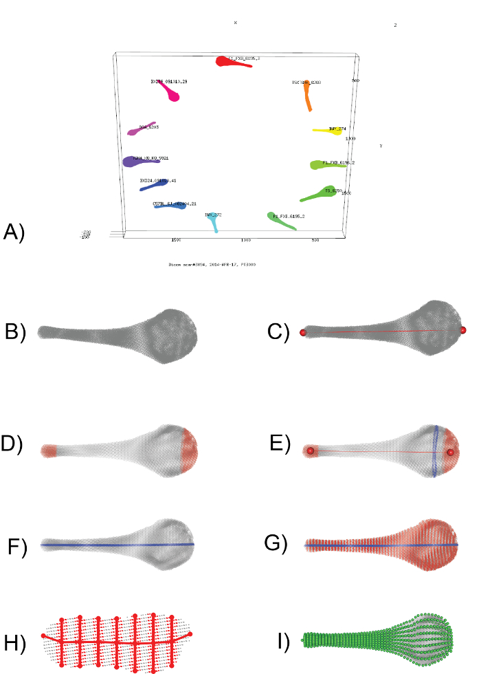
Figure 1: Visual Representation of the Computational Workflow (Protocol 4-6). (A) A screenshot from the 02_segment_dicoms.r script (Protocol 4), showing the assignment of distinct point clouds to individual specimens. (B) Enlarged view of one baculum, represented by a cloud of ~100K x-y-z points. (C) Identification of the two points furthest apart from each other (red spheres), used to define a new z-axis that runs proximal-distal through the bone (red line). (D) Sampling the proximal-most 10% and distal-most 10% of points (red points) provides a means to adjust for slight variance in the exact placement of the z-axis. (E) The centroids of the proximal-most 10% and distal-most 10% (red spheres) are used to define a new z-axis (red line). Then, a slice of points falling between 15.00-15.25% of this new z-axis (blue points) is taken to calculate the minimum bounding rectangle. The point cloud is rotated until the long side of the minimum bounding rectangle is parallel to a new x-axis. F) a slice of points running along the midline (blue points) is sampled and the proximal-most and distal-most point defined as a semi-landmark. G) 50 evenly spaced slices of points are sampled (red points), with H) showing one such slice. 16 points (red circles) are defined to capture the outline of each slice. I) When repeated across all slices, a total of 802 semi-landmarks (green spheres) define the structure and are used in all downstream morphometric applications. Please click here to view a larger version of this figure.
The critical steps in the above protocol are 1) dissecting the bacula, 2) gathering the microCT images, 3) converting the microCT output to a flat file of x-y-z coordinates, 4) segmenting out each specimen's point cloud, 5) transforming each specimen to a standardized coordinate system, and 6) defining semi-landmarks. These steps are easily modified to accommodate different objects.
These methods can likely be applied to any object that is essentially "rod-shaped", or at least not too curved. Objects that curve back on themselves to become "u-shaped" cannot be currently analyzed, because slicing (Figure 1G) would return points from different parts of the object. Such objects could be accommodated in the future by computationally straightening the object prior to slicing.
We have presented a general method for mathematically defining semi-landmarks from shapes that lack solid landmarks. These general methods have been modified to study the evolution of whale pelvic and rib bones16, which have very different shapes. Our computational methods for defining landmarks should be applicable to any series of x-y-z coordinates. We employed microCT scanning here, given the small size of mouse bacula14. For larger bones, such as the whale pelvic and rib bones, we employed a laser scanner that reconstructed the surface of the bones16. It is important to visually inspect all sets of semi-landmarks to verify the quality of the method. The main advantage of our computational methods is that they precisely quantify the size and shape variation, and preserve the correspondence between distinct regions of the object.
The authors have nothing to disclose.
Tim Daley and Andrew Smith provided many useful computational discussions during the early days; Tim Daley wrote the program rotate_translate_cylindrical necessary for Protocol 5. Computational resources were provided by the High Performance Computing Cluster at the University of Southern California. This work was supported by NIH grant #GM098536 (MDD).
Dissecting scissors | VWR | 470106-338 | Most sizes should work |
Dissecting Forceps, Fine Tip, Curved | VWR | 82027-406 | |
1.7 mL microcentrifuge tube | VWR | 87003-294 | |
Absolute Ethanol | Fisher Scientific | CAS 64-17-5 | To be diluted to 70% for dissections |
Floral Foam | Wholesale Floral | 6002-48-07 | |
uCT50 scanner | Scanco Medical AG, Bruttisellen, Switzerland |