Central and Divided Visual Field Presentation of Emotional Images to Measure Hemispheric Differences in Motivated Attention
Summary
This study compared central versus divided visual field presentations of emotional images to assess differences in motivated attention between the two hemispheres. The late positive potential (LPP) was recorded using electroencephalography (EEG) and event-related potentials (ERPs) methodologies to assess motivated attention.
Abstract
Two dominant theories on lateralized processing of emotional information exist in the literature. One theory posits that unpleasant emotions are processed by right frontal regions, while pleasant emotions are processed by left frontal regions. The other theory posits that the right hemisphere is more specialized for the processing of emotional information overall, particularly in posterior regions.
Assessing the different roles of the cerebral hemispheres in processing emotional information can be difficult without the use of neuroimaging methodologies, which are not accessible or affordable to all scientists. Divided visual field presentation of stimuli can allow for the investigation of lateralized processing of information without the use of neuroimaging technology.
This study compared central versus divided visual field presentations of emotional images to assess differences in motivated attention between the two hemispheres. The late positive potential (LPP) was recorded using electroencephalography (EEG) and event-related potentials (ERPs) methodologies to assess motivated attention. Future work will pair this paradigm with a more active behavioral task to explore the behavioral impacts on the attentional differences found.
Introduction
Several theories on lateralized processing have been posited for the two cerebral hemispheres. Among these include theories of emotional processing. The valence model1 proposes that the left hemisphere is specialized for pleasant emotions, while the right hemisphere is specialized for unpleasant emotions. The right hemisphere dominance hypothesis2 proposes that the right hemisphere is specialized for processing all emotional information compared to the left hemisphere. Finally, the Circumplex Theory3 proposes that in addition to frontal asymmetries for valence, the posterior regions of the right hemisphere are specialized for processing all high-arousing emotions. In order to test these lateralized theories of processing, methodologies that can differentiate processing between the two hemispheres must be used. While neuroimaging techniques can provide this information, they are often not readily accessible to most research scientists. Further, many standard cognitive paradigms, even when coupled with neuroimaging methodologies, do not isolate information processed within each hemisphere. Divided visual field (DVF) methodologies provide an avenue for behavioral and psychophysiological scientists to test lateralized theories of processing without the use of neuroimaging techniques.
DVF methodologies are based on the knowledge that a stimulus presented to one visual field is initially received and processed by the contralateral hemisphere4. DVF methodologies utilize lateralized presentations of stimuli at short intervals to allow one cerebral hemisphere to receive the information before the other5. As such, stimuli presented briefly to the right visual field are processed contralaterally by the left hemisphere, and stimuli presented to the left visual field are processed by the right hemisphere. In this manner, differences in initial processing of the information in a single hemisphere can be examined. For example, it is well established that the left hemisphere is specialized for processing linguistic information (for a meta-analysis see reference6). Research using DVF paradigms demonstrate increased processing speed when words are presented to the left hemisphere (i.e., displayed in the right visual field) compared to when presented to the right hemisphere.
In order to assess the processing differences between the two hemispheres, measures with finer temporal resolution than behavioral reaction times may be needed. Event-related potentials (ERPs) derived from human electroencephalography (EEG) data have a temporal resolution on the order of milliseconds (ms). As such, using ERP techniques in concert with DVF methodologies allows for a refined assessment of processing differences between the two hemispheres. Initially, central visual field (CVF) presentations of the stimuli can be used to replicate established ERP effects. Then, DVF presentations of the stimuli can be used to examine the unique contributions of each hemisphere to the propagation of these ERP effects. Of particular interest for the current study7, the late positive potential (LPP) has been identified as an ERP component sensitive to the emotional arousal of a stimulus8. Interestingly, the LPP has not been found to consistently differentiate between unpleasant and pleasant stimuli, but rather, responds equally to emotional stimuli relative to neutral stimuli. This study was designed to test the lateralized processing of emotion theories using the LPP as an index of motivated attention toward emotional stimuli between the two hemispheres.
Further, this study systematically examines both the valence and arousal dimensions of the emotion stimuli across early and late manifestations of the LPP. These stimulus manipulations in combination with both CVF and DVF stimulus presentations are unique to the literature, as they allow for examining the unique and interactive influences of valence, arousal, and hemisphere of processing on the propagation of the LPP. As such, the influence of immediacy for action signaled by unpleasant compared to pleasant stimuli, which should differentially engage motivated attention and thus the LPP, can be explored.
Protocol
All methods described here have been approved by the Internal Review Board for human subject research at the University of Kansas, Lawrence, KS.
1. Selecting Participants
- Use right-handed participants for DVF research. In rare cases (10%), left-handed individuals are lateralized for language processing in the right hemisphere, which would result in scalp-recorded ERP components with non-typical topographical distributions.
- Have participants complete the Edinburgh Handedness Inventory9 to determine strong right-handedness. Scores of eight or higher indicate strong right-handedness.
2. Stimuli
- Request a research copy of the International Affective Picture System (IAPS)10 via the Center for the Study of Emotion and Attention's website11. Select stimuli from the IAPS according to the specifications in steps 2.2-2.4. The IAPS comes with an image file for each stimulus and a tab-delimited text file containing the normed ratings of valence and arousal for each image.
- Use a spreadsheet program to view the norms and make the stimuli selections. For a complete list of the stimuli selected for O'Hare, Atchley, and Young (2016) see Table 1.
NOTE: This stimulus set provides norms for the rated valence and arousal of emotional stimuli. The norms for the stimuli were created via participant ratings on the Self-Assessment Mannequin10. This scale depicts a graphic figure that ranges from a frowning, unhappy figure to a smiling, happy figure for valence, and a relaxed, sleepy figure to an excited, wide-eyed figure for arousal. Valence is rated on a 9-point Likert scale with 1 equaling the most unpleasant (frowning, unhappy figure) and 9 equaling the most pleasant (smiling, happy figure). Arousal is also rated on a 9-point Likert scale with 1 equaling the least arousing (relaxed, sleepy figure) and 9 equaling the most arousing (excited, wide-eyed figure). The components of each image that evoke emotional responses are located centrally in each image.
- Use a spreadsheet program to view the norms and make the stimuli selections. For a complete list of the stimuli selected for O'Hare, Atchley, and Young (2016) see Table 1.
- Create three valence groups of images with 60 images in each group: unpleasant, pleasant and neutral, using the norms provided in the IAPS manual12.
- To do this, sort the IAPS images by their average valence rating. Unpleasant stimuli range in average valence rating from 1 to 3.99. Neutral stimuli range in average valence rating from 4 to 6.99. Pleasant stimuli range in average valence rating from 7 to 9. Each valence group must significantly differ from each other in average valence rating with no overlap in their ranges.
- Confirm that valence groups significantly differ from each other using independent samples t-tests13. Picture complexity across the image groups is not controlled as image complexity has not been found to influence the LPP14.
- Within both the unpleasant and pleasant valence stimuli, create high and medium arousal subgroups of 30 images each.
- Within the neutral valence stimuli, create medium and low arousal subgroups. High arousal subgroups range in average arousal ratings from 4.30 to 8.70 and do not significantly differ from each other on average arousal rating. Medium arousal subgroups range in average arousal ratings from 2.40 to 7.29 and do not significantly differ from each other on average arousal rating. The low arousal subgroup ranges in average arousal ratings from 1.4-5.44.
- Once the stimuli have been selected, test them (via t-tests)13 to ensure the stimuli groups are reliably different.
NOTE: Each of the arousal subgroups (high, medium, and low) must significantly differ from each other in average arousal rating, but arousal subgroups within a valence group do not significantly differ from each other in valence. This allows for examination of 1) valence effects alone, 2) arousal effects alone, and 3) interactive effects between valence and arousal. - Using an image-editing software program, resize the final stimulus images to ensure that they will be presented at 17.06 horizontal and 10.85 vertical degrees of visual angle on the stimulus-presentation monitor.
- Calculate the visual angle (V) using the formula, V = 2arctan(S/2D)15, where S = the height or width of a visual object, and D = the distance from the viewer's pupil to the visual object. The size of the stimulus images will depend upon the distance between the participant's pupils and the stimulus-presentation monitor (D).
- Create mask stimuli for backward masking of the image stimuli. Mask stimuli consist of an array of backward slashes (i.e., "") that match the spatial dimensions of the images. Create a textbox that has the same dimensions in pixels as the image stimuli in an image-editing software program. Enter backward slashes into the textbox until they fill the entire space without changing the dimensions specified. Save this textbox as an image to create the mask stimulus.
- For the DVF paradigm, create the image-presentation slides to be loaded into the stimulus presentation software.
- In an image-editing software program, center a fixation mark ("+") in the middle of the image. Place your first stimulus image centered vertically with its right edge 3° of visual angle to the left of the fixation mark.
- Create a brown rectangle with the same dimensions as the stimulus image and place it also centered vertically with its left edge 3-degrees of visual angle to the right of the fixation mark. Save this arrangement as the left visual field presentation of this stimulus image.
- Switch the location of the stimulus image and the brown rectangle and save this arrangement as the right visual field presentation of this stimulus image. Do this for all stimulus images (Figure 1).
- For the DVF paradigm, create the mask-presentation slides to be loaded into the stimulus presentation software in the same manner as was done for the image-presentation slides. Place the mask image on both sides of the fixation mark with both inner edges 3-degrees of visual angle from the fixation mark (Figure 2). Save this arrangement as the mask stimulus for the DVF paradigm.
3. Experimental Equipment
- Use Silver-Silver chloride (Ag-AgCl) active-electrodes or other EEG electrodes to record EEG from scalp positions according to the international 10-20 system16. Position one additional electrode above and another below the right eye to record vertical eye movements.
- Use EEG acquisition software for data acquisition with a sampling rate of 250-500 Hz, depending upon equipment specifications. For a detailed consideration of EEG acquisition parameters see Luck (2014)17.
- Present stimuli via an stimulus-presentation software package18 on a computer with a mirrored 24-inch stimulus-presentation liquid crystal display monitor (1,920 x 1,200 resolution) that is in a separate, electrically-shielded, and sound attenuated room. Place only the mirrored monitor within the shielded room, while keeping the computer out of the experimental room reduces electrical noise. Sound attenuation reduces the occurrence of auditory-evoked potentials in the EEG data. The stimulus-presentation software package must allow for users to set the presentation durations and screen locations of stimuli.
4. Preparing the Participant
- Have participants complete informed, written consent prior to providing any data.
- Have participants complete a demographic survey to provide sex, age, handedness, native language, vision, and neurological history. Collect sex and age for reporting in final study dissemination. Use all other demographic information to determine if the participant meets the criteria for inclusion in the study: right-handed (assessed via the Edinburgh Handedness Inventory), native English speaker collected via self-report (or native to the language used in the study instructions), normal or correct-to-normal vision, and no history of neurological trauma.
- Apply EEG electrodes onto the participant. Any EEG montage that covers occipital-parietal regions of the scalp is appropriate for recording the LPP response.
- Seat participants in a dark, electrically-shielded, sound-attenuated room. Use a chin rest to stabilize the head and minimize movement. Position the chin rest the correct distance away from the stimulus-presentation monitor to maintain the D variable used in the visual angle calculations. Place a keyboard (or response box) in front of the participant for response collection via their right hand.
- Check the data signal to ensure that all channel impedances are less than 50 kiloohms17.
- Instruct participants to passively view the image stimuli without shifting their eyes away from the center of the screen. Display a fixation mark ("+") at the center of the screen to help participants fixate17. Instruct the participant that there will be a recognition quiz following each block of images, so it is important that they pay attention. Each participant only completes the CVF or the DVF paradigm, creating a between-subjects design.
NOTE: Both CVF and DVF paradigms can be conducted on the same participant to create a within-subjects design. If this is done, counterbalance the order of the two paradigms to control for any familiarity effects with the stimuli.
5. Central Visual Field (CVF) Paradigm
NOTE: In the CVF paradigm, randomly present image stimuli at the center of the screen. Each trial consists of a 500 ms central fixation ("+") followed by a 150 ms presentation of the stimulus, followed by a backward mask that varies randomly in presentation duration between 2,000-4,000 ms. Jittered presentation duration for the mask serves to reduce any anticipatory ERP responses to the onset of the next trial20.
- To specify the presentation durations and stimuli locations create separate presentation slides for the fixation, the stimulus images, and the mask stimulus in your stimulus-presentation software.
- For the presentation of the fixation mark, specify the presentation of the plus sign symbol ("+") centered both vertically and horizontally and set the duration to 500 ms. This can be done through the properties for this slide.
- For the presentation of the stimulus, enter the image file names for the stimuli into a matrix or list object.
- On the image-presentation slide, place an image object centered both vertically and horizontally, and link this object to the list of image file names to load the image stimuli. Set the matrix or list object with the image file names to randomly select from the list without replacement of already selected stimuli. Set the duration of the image-presentation slide to 150 ms.
- For the mask-presentation slide, again place an image object centered both vertically and horizontally. This object can be directly linked to the mask image file by entering the file name in its properties. Set the duration of the mask-presentation slide to randomly vary between 2,000-4,000 ms.
- Present image stimuli in four experimental blocks of 45 trials each (180 trials total). Each block has an equal number of stimuli from the valence/arousal conditions. This can be accomplished by creating four separate matrices or list objects with the image file names, each containing 7-8 images from each valence-arousal group (e.g., in list 1 there can be 7 high-arousing unpleasant images and in list 2 there can be 8 high-arousing unpleasant images). Participants passively view the image stimuli on each trial.
- Following each block, give a 10-item recognition test to ensure participants pay attention during the passive viewing portion of the study. Display six items on the recognition test from the preceding block and four items that are new. Select these six items so that they represented all categories of valence and arousal. Have participants respond via key press using their right hand indicating which stimuli they previously viewed.
6. Divided Visual Field (DVF) Paradigm
NOTE: The DVF paradigm is identical to the CVF paradigm, including the size of the image stimuli, except present each image stimulus laterally, to the left or right of the fixation mark using the image-presentation slides created in step 2.7 (see Figure 3)4.
- Present each image once in the left visual field and once in the right visual field. Present all stimuli in a fully randomized order.
- As each stimulus is presented twice, double the number (8) of experimental blocks and recognition tests for a total of 360 trials.
- Pair each image stimulus with the simultaneous presentation of a solid brown rectangle identical in stimulus dimensions on the opposite side of the fixation. This is done to reduce reflexive saccades to the stimulus. Additionally, the presentation duration of 150 ms is shorter than most saccade latencies21, meaning that if the participant shifts his/her eyes to the stimulus, it will be masked before the participant can fixate on it22.
- Present each stimulus and its paired brown rectangle with their inside edge 3° of visual angle from the fixation. This is done to assure that the stimuli fall entirely within the regions of the retinas that are processed by only one hemisphere4.
- Backward mask both the stimulus and the brown rectangle using the same criteria and procedure as was done in the CVF paradigm20.
7. Data Analysis
- Remove any participant scoring less than 50 percent (chance) on the recognition test from the data, as it cannot be assured that he/she was paying attention to the stimuli.
- Preprocess and analyze EEG data using an EEG software package23. Filter data offline with a continuous 0.01-30 Hz bandpass, mark data fluctuating 200 μv within a 100 ms time window as bad, correct eye blink artifacts using an average template generated from each individual participant, manually remove horizontal eye shifts from the data following visual inspection, and rereference data using the common average rereference24,25.
- Compute epochs of 1,000 ms after the onset of the stimuli according to a 200 ms pre-stimulus baseline26.
- Use visual inspection of the waveforms and the ERP literature to determine the topography of the LPP27. In this study, the LPP centered on channel CPz. In this case, average channels CPz, Pz, Cz, CP1 and CP2 together to create a representation of the LPP.
- In the DVF data, conduct a laterality analysis comparing the LPP amplitude across left occipital-parietal channels and right occipital-parietal channels to ensure that the DVF presentations did not shift the typical topography of the LPP component. Conduct paired-samples t-tests between channel pairs CP1 and CP2, CP3 and CP4, C1 and C2, C3 and C4, P1 and P2, and P3 and P4 respectively to ensure that they do not significantly differ from each other on average amplitude.
- As the LPP is a long, sustained component, extract two different LPP epochs: early (400-700 ms post-stimulus onset) and late (700-1,000 ms post-stimulus onset).
- Analyze the CVF LPP data via a 3 (Valence: unpleasant, pleasant, and neutral) by 2 (Epoch: early and late) within-groups analysis of variance (ANOVA) to ensure that the typical LPP effect of emotional stimuli generating larger LPP responses than neutral stimuli is present. This analysis is done to affirm that the stimuli were processed normally.
- To examine the interactive effects of valence and arousal on the LPP conduct a 2 (Valence: unpleasant and pleasant) by 2 (Arousal: high and low) by 2 (Epoch: early and late) within-groups ANOVA on the CVF LPP data.
- To examine the effects of hemisphere of presentation, conduct the ANOVA specified in section 7.8 with the additional factor of Hemisphere: left and right on the DVF LPP data.
Representative Results
To replicate previous research on the LPP, both LPP responses to unpleasant and pleasant images should be larger than LPP responses to neutral images. This is confirmed by the CVF analysis, which finds the LPP in the early epoch to be significantly larger to unpleasant (M = 1.90 μv) and pleasant (M = 1.71 μv) images compared to neutral images (M = 0.72 μv), but unpleasant and pleasant images are not found to be significantly different from each other. Interestingly, in the late epoch, the LPP is found to be larger for unpleasant (M = 1.19 μv) compared to pleasant images (M = 0.56 μv).
To examine the effects of hemisphere of processing on the LPP response to emotional images, differences in the LPP between the hemispheres of presentation are of interest. In this study, the LPP is found to be larger in the early epoch compared to the late epoch for all image presentations except for high-arousing unpleasant images presented to the left hemisphere. These images are not found to elicit significantly different LPP responses between the two epochs (see Table 2). In other words, the LPP response to high-arousing unpleasant images is sustained in comparison to medium-arousal unpleasant images and all pleasant images. This finding can be used to inform the theories of lateralized emotion processing. In particular, these data support theories of emotion processing that propose the right hemisphere is specialized for general emotion identification, while the left hemisphere is specialized for creating specific action plans in response to emotional stimuli28. Here, it appears that the left hemisphere engages high-arousing unpleasant images for longer, possibly to address the need for action or not.
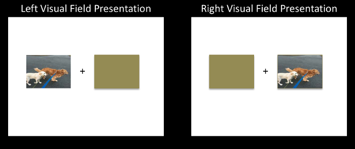
Figure 1: A schematic of the Divided Visual Field (DVF) paradigm. Each trial consists of a centrally presented fixation ("+") for 500 ms, followed by a lateralized stimulus presentation that is paired with a brown rectangle for 150 ms, followed by a backward mask for a random interval between 2,000-4,000 ms. Please click here to view a larger version of this figure.
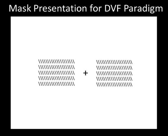
Figure 2: Mask Presentation for DVF Paradigm. Please click here to view a larger version of this figure.
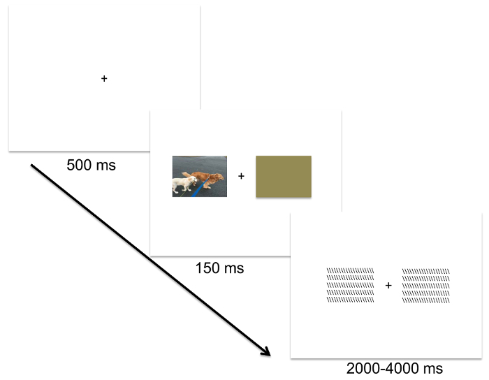
Figure 3: The DVF paradigm is identical to the CVF paradigm, including the size of the image stimuli, except present each image stimulus laterally, to the left or right of the fixation mark using the image-presentation slides. Please click here to view a larger version of this figure.
| High-Arousing Unpleasant | Medium-Arousing Unpleasant | High-Arousing Pleasant | Medium-Arousing Pleasant | Medium-Arousing Neutral | Low-Arousing Neutral |
| 3500 | 9000 | 8300 | 1600 | 1080 | 2271 |
| 6360 | 2750 | 4607 | 2341 | 1030 | 2280 |
| 9300 | 9432 | 5629 | 7230 | 2810 | 7234 |
| 3150 | 6311 | 8034 | 1590 | 8010 | 7700 |
| 6315 | 9265 | 4608 | 2345 | 9913 | 2210 |
| 3400 | 9320 | 8400 | 1999 | 6930 | 2221 |
| 6230 | 2276 | 8180 | 1463 | 7560 | 5120 |
| 6300 | 3181 | 8490 | 4622 | 1303 | 7590 |
| 2683 | 3051 | 4290 | 1500 | 1112 | 4233 |
| 9620 | 9911 | 8170 | 2331 | 6900 | 2516 |
| 6370 | 9420 | 8080 | 7352 | 2780 | 4000 |
| 6200 | 3061 | 8470 | 2224 | 2690 | 5534 |
| 6313 | 6243 | 8370 | 8497 | 5535 | 2490 |
| 9800 | 9006 | 8501 | 8210 | 7211 | 7180 |
| 9921 | 9340 | 4220 | 2650 | 1935 | 2830 |
| 9910 | 9561 | 8190 | 2310 | 6314 | 9070 |
| 9810 | 3300 | 4676 | 4610 | 7820 | 7224 |
| 6560 | 3101 | 4690 | 1721 | 1101 | 2383 |
| 6212 | 3180 | 4687 | 8090 | 7503 | 2272 |
| 6570 | 2205 | 4659 | 2352 | 5970 | 7920 |
| 6540 | 9280 | 4689 | 5460 | 9582 | 7031 |
| 6415 | 9415 | 4670 | 2303 | 1240 | 9210 |
| 6821 | 9342 | 8186 | 2208 | 9402 | 9401 |
| 9050 | 9220 | 4680 | 8540 | 3210 | 2480 |
| 6260 | 9560 | 8030 | 2395 | 1390 | 7595 |
| 2730 | 9140 | 5470 | 4641 | 2230 | 2590 |
| 6510 | 9421 | 4660 | 4700 | 1945 | 7025 |
| 6312 | 9301 | 8200 | 5480 | 1230 | 2215 |
| 9600 | 9181 | 5621 | 7260 | 2410 | 7186 |
| 9250 | 9435 | 8185 | 8461 | 9411 | 2441 |
Table 1: Stimuli ID numbers for selected stimuli for O'Hare, Atchley and Young (2016) from the IAPS sorted by arousal and valence groups.
| Left Hemisphere | Right Hemisphere | |||
| Early Epoch | Late Epoch | Early Epoch | Late Epoch | |
| High-Arousing Unpleasant | 2.839 | 2.629 | 2.48 | 0.968* |
| High-Arousing Pleasant | 2.521 | 1.783* | 3.03 | 1.8* |
Table 2: Mean LPP amplitudes for the DVF analysis.
Discussion
In this study, manipulations of stimulus valence and arousal were used with the DVF paradigm to test theories of lateralized processing of emotion as they apply to the motivated attention network. However, DVF methodologies can be used to explore any lateralized processing of visual information. What is critical when using DVF paradigms is the control of the stimuli presentation to ensure that the information is isolated to one hemisphere for initial processing. There are several key steps to the DVF paradigm that contribute to this aspect of the research.
First, participants are instructed to keep their eyes fixated at the center of the screen. A fixation mark, bilateral dummy stimulus (or placeholder), and a head-stabilizing chin rest are used to assist participants with maintaining this fixation. Nonetheless, participants will occasionally shift their gaze to the laterally presented stimuli. Trials in which an eye shift occurred should not be included in the analyses, as fixating on the stimulus allows both hemispheres to receive the information simultaneously. In ERP research, horizontal eye shifts can be detected in the EEG data, and those trials can be removed. In behavioral research, it may be necessary to continuously use a mirror or eye tracking to monitor eye movements.
In addition to controlling for eye shifts, stimuli need to be presented in a manner that prevents bilateral processing. To do this, it is recommended that stimuli appear no less than 3° of visual angle from the fixation. It is also important not to present stimuli too laterally, where visual acuity will decline. Stimuli extending beyond 10° of visual angle from the fixation are at risk for low visual acuity (see reference4 for a detailed discussion). Additionally, stimuli need to be presented below the average express saccade latency (150 ms)21. Express saccades are reflexive eye shifts to changes in the visual field, such as a stimulus appearing. Additionally, displaying a backward mask following the offset of the stimulus disrupts any early, bilateral processing of the stimulus22. Presenting the mask stimulus immediately after the experimental stimulus does add another visual stimulus to the ERP window, possibly contaminating the resulting ERP components. However, consistently using the mask stimulus across all trials of interest still allows for the examination of the effects of stimulus variables, such as valence and arousal, beyond these basic visual processing effects, as they should cancel out across the comparison of conditions.
EEG and ERPs are one way to assess the impact of lateralized processing of stimuli. It is important when using these methodologies to know if the ERP components you intend to analyze are subject to shifting their topographies following lateralized presentations of stimuli. For the LPP, previous DVF studies did not find topographical shifts29,30, but other ERP components may be sensitive to visual field side of presentation. Larger ERP amplitudes are indices of additional processing resources being used to process any given presentation of a stimulus. For example, in this study, larger LPP responses were found in the late epoch for high-arousing unpleasant images presented to the left hemisphere. This is interpreted as the left hemisphere engaging in more elaborate processing of these stimuli compared to the right hemisphere or compared to pleasant or neutral stimuli.
Behavioral tasks can also be used to assess the effects of lateralized processing of stimuli. In this case, changes in accuracy or reaction time in response to the lateralized presentations of stimuli can be interpreted as differences in the efficiency of the two hemispheres in processing that type of information. For example, both accuracy and reaction time differences between hemispheres of presentation have been found in DVF semantic priming tasks31.
DVF paradigms can be limited in that the presentation duration of the stimuli must be kept below 150 ms to prevent saccades and bilateral processing. As such, complex stimuli that require longer processing may be inappropriate for this methodology. Further, DVF paradigms can only be used to make inferences about processing in an entire cerebral hemisphere. Investigating processing within specific brain regions at a finer level than cerebral hemisphere is not possible with DVF techniques alone. If specific brain regions are part of the research question, neuroimaging or ERP techniques must be used in concert with the DVF paradigm.
DVF paradigms provide an avenue for studying lateralized processing in the brain without the need for neuroimaging equipment. This makes the study of the brain more accessible to all researchers. In the study of lateralized processing of emotional information, future studies that pair DVF presentations of systematically controlled emotional stimuli with a behavioral task can further explore the unique contributions of each cerebral hemisphere to our emotional experience.
Disclosures
The authors have nothing to disclose.
Acknowledgements
None.
Materials
| 64-channel Ag-AgCl active electrodes | Cortech Solutions | DA-AT-ESP32102064A/DA-AT-ESP32102064B | EEG electrodes for data collection |
| ActiveTwo Base System | Cortech Solutions | DA-AT-BCBS | Digitizes and ampliphies EEG data at 500 Hz |
| E-Prime Professional 2.0 | Psychology Software Tools | NA | Stimulus presentation software, available at https://www.pstnet.com/eprime.cfm |
| CURRY 7.0 | Compumedics Neuroscan | NA | EEG/ERP data processing and analysis, available at http://compumedicsneuroscan.com/products/by-name/curry/ |
References
- Ali, N., Cimino, C. R. Hemispheric lateralization of perception and memory for emotional verbal stimuli in normal individuals. Neuropsychology. 11 (1), 114-125 (1997).
- Cacioppo, J. T., Crites, S., Gardner, W. L. Attitudes to the right: evaluative processing is associated with lateralized late positive event-related brain potentials. Pers Soc Psycho B. 22 (12), 1205-1219 (1996).
- Heller, W., Nitschke, J. B., Miller, G. A. Lateralization in emotion and emotional disorders. Curr Dir in Psychol Sci. 7 (1), 26-32 (1998).
- Beaumont, J. G., Young, A. W. Functions of the right cerebral hemisphere. Methods for studying cerebral hemispheric function. , 114-146 (1983).
- Bourne, V. J. The divided visual field paradigm: methodological considerations. Laterality. 11 (4), 373-393 (2006).
- Vigneau, M. Meta-analyzing left hemisphere language areas: phonology, semantics, and sentence processing. NeuroImage. 30, 1414-1432 (2006).
- O’Hare, A. J., Atchley, R. A., Young, K. M. Valence and arousal influence the late positive potential during central and lateralized presentation of images. Laterality. , 1-19 (2016).
- Olofsson, J. K., Nordin, S., Sequeira, H., Polich, J. Affective picture processing: an integrative review of ERP findings. Biol Psychol. 77 (3), 247-265 (2008).
- Oldfield, R. C. The assessment and analysis of handedness: The Edinburgh inventory. Neuropsychologia. 9, 97-113 (1971).
- Lang, P. J., Bradley, M. M., Cuthbert, B. N., Lang, P. J., Simons, . R. F., Balaban, M., Simons, R. Motivated attention: affect, activations, and action. Attention and orienting: Sensory and motivational processes. , 97-135 (1997).
- Lang, P. J., Bradley, M. M., Cuthbert, B. N. International affective picture system (IAPS): affective ratings of pictures and instruction manual. Technical Report A-8. , (2008).
- Nolan, S. A., Heinzen, T. E. Hypothesis testing with t tests: comparing two groups. Statistics for the Behavioral Sciences. , 382-421 (2008).
- Bradley, M. M., Hamby, S., Low, A., Lang, P. J. Brain potentials in perception: picture complexity and emotional arousal. Psychophysiology. 44, 364-373 (2007).
- Mccready, D. On size, distance, and visual angle perception. Percept Psychophys. 37 (4), 323-334 (1985).
- Jasper, H. H. Report of the committee on methods of clinical examination in electroencephalography: 1957. Electroen Clin Neuro. 10 (2), 370-375 (1958).
- Luck, S. J. . Basic principles of ERP recording. An Introduction to the Event-Related Potential Technique. , 147-184 (2014).
- Luck, S. J. The design of ERP experiments. An Introduction to the Event-Related Potential Technique. , 119-146 (2014).
- Woodman, G. F. A brief introduction to the use of event-related potentials (ERPs) in studies of perception and attention. Atten Percept Psychophys. 72 (8), 2031-2046 (2010).
- Carpenter, R. H. S. . Movements of the eyes. , (1988).
- Young, K. M., Atchley, R. A., Atchley, P. Offset masking in a divided visual field study. Laterality. 14 (5), 473-494 (2009).
- Compumedics Neuroscan. . CURRY 7 [computer software]. , (2008).
- Luck, S. J. Artifact rejection and correction. An Introduction to the Event-Related Potential Technique. , 185-218 (2014).
- Luck, S. J. Baseline correction, averaging, and time-frequency analysis. An Introduction to the Event-Related Potential Technique. , 249-282 (2014).
- Kappenman, E. S., Luck, S. J., Luck, S. J., Kappenman, E. S. ERP components: the ups and downs of brainwave recordings. The Oxford Handbook of Event-Related Potential Components. , 3-30 (2012).
- Hajcak, G., Weinberg, A., MacNamara, A., Foti, D., Luck, S. J., Kappenman, E. S. ERPs and the study of emotion. The Oxford Handbook of Event-Related Potential Components. , 441-474 (2012).
- Hugdahl, K. Lateralization of cognitive processes in the brain. Acta Psychol. 105 (2-3), 211-235 (2000).
- Kayser, J. Neuronal generator patterns at scalp elicited by lateralized aversive pictures reveal consecutive stages of motivated attention. NeuroImage. 142 (15), 337-350 (2016).
- Kayser, J. Event-Related Potential (ERP) asymmetries to emotional stimuli in a visual half-field paradigm. Psychophysiology. 34, 414-426 (1997).
- Smith, E. R., Chenery, H. J., Angwin, A. J., Copland, D. A. Hemispheric contributions to semantic activation: a divided visual field and event-related potential investigation of time-course. Brain Res. 1284, 125-144 (2009).
