An EEG-fMRI multimodal imaging method, known as the spatiotemporal fMRI-constrained EEG source imaging method, is described here. The presented method employs conditionally-active fMRI sub-maps, or priors, to guide EEG source localization in a manner that improves spatial specificity and limits erroneous results.
Electroencephalography (EEG) and functional magnetic resonance imaging (fMRI) are two of the fundamental noninvasive methods for identifying brain activity. Multimodal methods have sought to combine the high temporal resolution of EEG with the spatial precision of fMRI, but the complexity of this approach is currently in need of improvement. The protocol presented here describes the recently developed spatiotemporal fMRI-constrained EEG source imaging method, which seeks to rectify source biases and improve EEG-fMRI source localization through the dynamic recruitment of fMRI sub-regions. The process begins with the collection of multimodal data from concurrent EEG and fMRI scans, the generation of 3D cortical models, and independent EEG and fMRI processing. The processed fMRI activation maps are then split into multiple priors, according to their location and surrounding area. These are taken as priors in a two-level hierarchical Bayesian algorithm for EEG source localization. For each window of interest (defined by the operator), specific segments of the fMRI activation map will be identified as active to optimize a parameter known as model evidence. These will be used as soft constraints on the identified cortical activity, increasing the specificity of the multimodal imaging method by reducing cross-talk and avoiding erroneous activity in other conditionally active fMRI regions. The method generates cortical maps of activity and time-courses, which may be taken as final results, or used as a basis for further analyses (analyses of correlation, causation, etc.) While the method is somewhat limited by its modalities (it will not find EEG-invisible sources), it is broadly compatible with most major processing software, and is suitable for most neuroimaging studies.
Electroencephalography (EEG) and functional magnetic resonance imaging (fMRI) can be viewed as neuroimaging modalities with complementary features. FMRI captures brain activity with large temporal scale, as hemodynamic signals indirectly measure the underlying neuronal activity with a poor temporal resolution (on the order of seconds)1,2. In contrast, EEG directly measures the dynamic electrophysiological activity of the brain with a very high temporal resolution (millisecond level), but poor spatial resolution3,4. These properties have led to multimodal approaches designed to optimize the favorable aspects of each individual method5. Simultaneous use of EEG and fMRI allows for the excellent temporal resolution of EEG to be combined with the high spatial accuracy of fMRI to overcome the limitations associated with unimodal fMRI or EEG.
Methods for EEG and fMRI integration begin with fMRI-informed EEG source localization6,7. This technique utilizes fMRI-derived spatial information to improve EEG source localization, however, one drawback is the potential spatial bias caused by the application of fMRI as a "hard-constraint" — fMRI-derived spatial information is considered an absolute truth. This poses two large issues that must be reconciled6–8. First, it must be considered that the use of a static map of Blood Oxygen Level Dependent (BOLD) contrasts may inadvertently strengthen any erroneous activity that falls within it, while damping true activity outside of it. Second, crosstalk from sources occurring outside of the BOLD activation map may influence the presentation of true activity within the results or cause erroneous activity. Despite this, the use of the high spatial resolution of fMRI to provide prior spatial knowledge remains a favorable solution5, as the modeling of the EEG inverse problem can be constrained both in the anatomical and functional senses.
In this paper, we demonstrate a spatiotemporal fMRI-constrained EEG source imaging approach that addresses the issue of temporal mismatch between EEG and fMRI by calculating the optimal subset of fMRI priors based on a hierarchical Bayesian model9. FMRI-priors are computed in a data-driven manner from particular windows of interest in the EEG data, leading to time-variant fMRI constraints. The proposed approach utilizes the high temporal resolution of EEG to compute a current density mapping of the cortical activity, informed by the high spatial resolution of fMRI in a time-variant, spatially selective manner that accurately images dynamic neural activity.
The protocol presented here was designed and performed in accordance with all guidelines for ethical human research as set forth by the respective Institutional Review Boards of the University of Houston and the Houston Methodist Research Institute.
1. Simultaneous EEG/fMRI Recording
2. Structural MRI Data Analysis and Forward Model Generation
3. Functional MRI Data Analysis
4. EEG Data Analysis
NOTE: Details in this section may be specific to the software used (See Table of Materials for more details). Please refer to the appropriate documentation if using different software packages.
5. Spatiotemporal fMRI Constraints — EG Source Imaging
EEG source localization at the basic level involves the solving of the forward and inverse problem. The components required to build and solve the forward problem are shown in Figure 5C. Using a subject-specific T1 image, three layers — brain, skull, and skin — were segmented and meshed. These layers served as the inputs to generate the BEM model. Similarly, the subject's grey-matter layer was segmented from the structural MRI and used to construct the source space. EEG sensor locations were co-registered onto the head model using a series of rigid geometrical transformations. When constructed, the forward model represents how electrical activity originating from any location on the source space would give rise to the potential measurements at each EEG sensor location on the scalp.
fMRI provides 3D images of brain functional activity with excellent spatial resolution and accuracy. Conventional fMRI analysis follows the GLM methods to identify the brain voxels significantly activated by a certain task. The typical result of this analysis is an fMRI activation map: a single brain map highlighting active voxels, which can be projected onto the gray matter surface, as shown in Figure 6A. We further divide the obtained activation maps into sub-maps, each acting as a potential spatial prior for localizing the scalp potentials measured by EEG in any particular time window (Figure 6B). Figure 8 represents the focused schematic of the spatiotemporal fMRI constrained source analysis described above. Only the appropriate partial set of the fMRI activation map is used to generate the EEG source reconstruction for the corresponding EEG data segment at the specified window size. As all EEG time-windows are analyzed, a complete reconstruction of the cortical activity is achieved in a spatiotemporally specific fashion that alleviates the spatial bias of applying the same fMRI priors at all EEG time points.
We further demonstrated a successful application of the spatiotemporal fMRI constrained source analysis method when applied to a visual/motor activation task study9, in which the sequence of brain activity from visual input to motor output was recovered with high spatiotemporal accuracy (Figure 9). While there is some dependence on the user's choice of window size, the reconstructed source imaging results were generally robust to moderate changes, as shown in Figure 10. To this end, the window size should be selected by the experimenter to best fit their particular study (i.e., a window size too large could prove to be erroneous for rapid activity or oscillations, while a window size too short may miss lower frequency signals) (Figure 10).
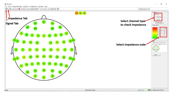
Figure 1: Scalp EEG impedance checking. Screenshot of the Recorder software user-interface, with arrows pointing to key icons in protocol step 1.2. Please click here to view a larger version of this figure.
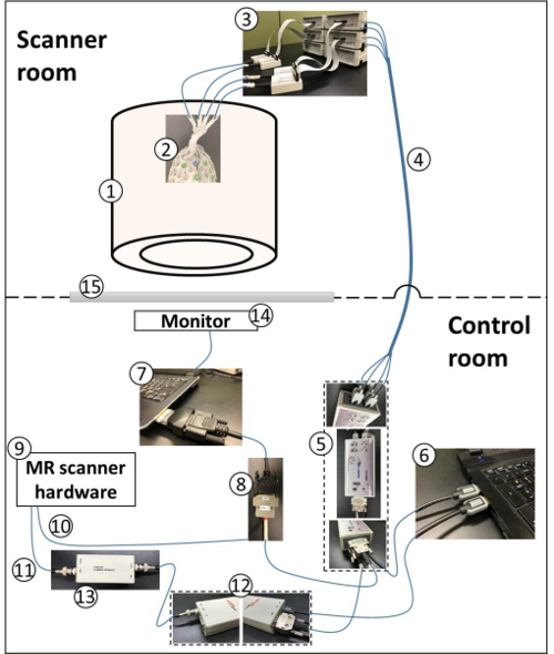
Figure 2: Schematic of simultaneous EEG/fMRI recording hardware setup — not drawn to scale. (1) Scanner; (2) participant wearing gelled EEG passive cap; (3) EEG amplifiers and Power Pack connected to the EEG cap; (4) optical fiber cables connecting the amplifiers to the USB 2 Adapter (also known as a BUA); (5) The BUA, an interface between amplifiers and the recording computer; (6) data acquisition computer; (7) Paradigm presentation computer, equipped with an express card to output event timing markers; (8) Transistor-transistor logic (TTL) trigger cable, delivering event timing markers from the presentation computer and the MR-scanner hardware to the BUA; (9) MR scanner hardware to provide timing markers at the start of (10) a new fMRI slice/volume acquisition and (11) clock synchronization signal; (12) Clock synchronization device, which provides synchronization between the clock of EEG amplifiers and the MR-scanner clock; (13) Interface module, interfacing between the MR-scanner and the clock synchronization device; (14) Monitor for the visual display of the experimental paradigm; (15) Glass window for viewing the scanner room from the control room. Please click here to view a larger version of this figure.
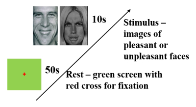
Figure 3: Experimental Paradigm. The subject was shown a series of visual stimuli, belonging to one of two categories: pleasant-face and unpleasant-face12. In each trial, a 50 s green screen baseline was first shown, followed by a randomly selected 10 s visual stimulus. The subject was to squeeze a rubber ball with his/her right hand for the entire duration of the stimulus shown, if the image was perceived as an unpleasant-face. Please click here to view a larger version of this figure.
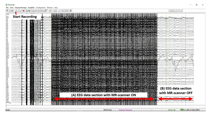
Figure 4: Screenshot of the EEG data recording. A representative section of the EEG data during the recording process. (A) Period of EEG data with fMRI pulse-sequence in effect, MR-scanner artifacts are pronounced. (B) Period of EEG data without fMRI pulse-sequence, no obvious MR-scanner artifacts are visible. Please click here to view a larger version of this figure.
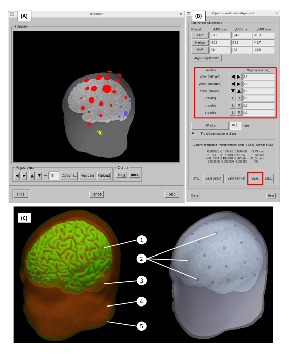
Figure 5: The forward model generation. (A) Alignment of EEG electrodes onto the head model space. Red and blue circles represent digitized EEG sensor locations, yellow circles represent the digitized EEG fiducial points: nasion, left preauricular, and right preauricular. (B) Options for the sensor alignment process, including manual transformation, such as the translation and rotation of the EEG sensor space (protocol step 2.4). (C) Subject specific BEM model generated, including 3 compartments: (3) brain, (4) skull, and (5) skin. The distributed source space on the surface of the (1) gray matter layer. (2) EEG sensor locations are aligned on the model. Please click here to view a larger version of this figure.
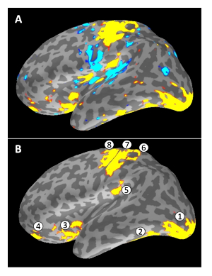
Figure 6: fMRI activation map and the extraction of regions of interest. (A) fMRI activation map shown on inflated surface for ease of inspection. Regions color coded in red and yellow are significantly activated (p-corrected<0.05). (B) 8 representative regions of interest extracted from the fMRI activation map. Note the atlas-based separation of motor activity into 3 priors. Please click here to view a larger version of this figure.
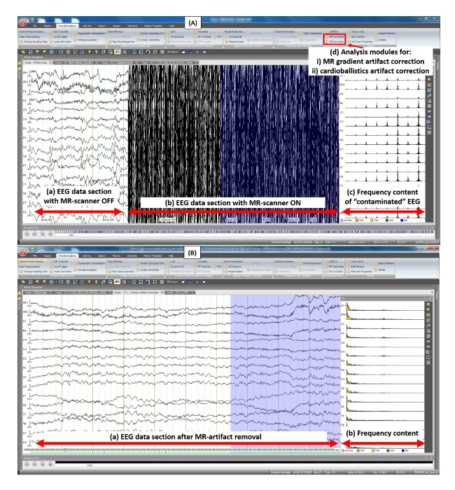
Figure 7: Screenshot of the Analyzer software user-interface — removal of MR-scanner artifacts.(A) Before scanner artifact correction: (a) EEG data section before the start of fMRI pulse-sequence; (b) EEG data section during fMRI pulse-sequence in effect, scanner artifacts are clearly visible; (c) the frequency content (FFT) of data section in (b); (d) Analyzer software's built-in analysis modules for scanner gradient-artifact correction and cardioballistic artifact correction. (B) After scanner artifact correction: (a) EEG data section after removal of MR-scanner artifacts; (b) the frequency content (FFT) of data section in (a). Please click here to view a larger version of this figure.
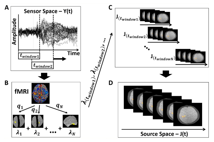
Figure 8: Overall schematic of the analysis process. (A) EEG data processing and window size selection. (B) fMRI data analysis, followed by the extraction of regions of interest to be used as spatial priors for the source analysis. (C) Source analysis performed at each EEG segment, specified by window sizes and percent overlap. (D) Complete reconstructed cortical activity over the time-course of interest. Please click here to view a larger version of this figure.
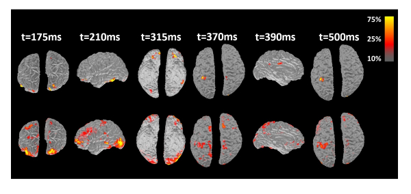
Figure 9: Reconstructed cortical activity of one representative subject underwent visual/motor activation paradigm. Source reconstruction results from contrasting two methods: spatiotemporal fMRI constrained (top) and time-invariant fMRI constrained source imaging (bottom). Figure reproduced with permission from reference9. Please click here to view a larger version of this figure.
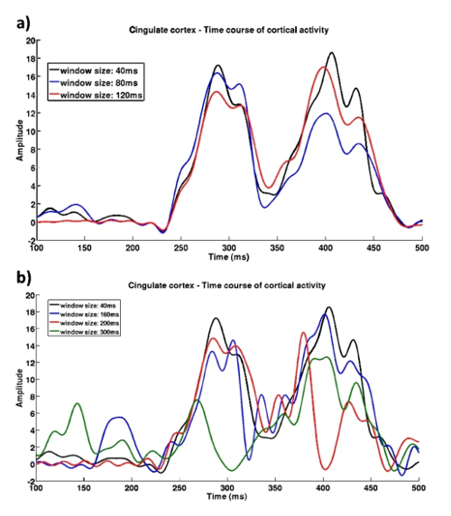
Figure 10: Reconstructed activity time-course at the cingulate cortex using different window sizes. (a) Activity time-courses reconstructed using smaller window sizes showed very similar results (correlation R >0.95). (b) Using larger window sizes resulted in high disparity (R <0.7). Figure reproduced with permission from reference9. Please click here to view a larger version of this figure.
We have shown here the necessary steps to use the spatiotemporal fMRI constrained source analysis method for EEG/fMRI integration analysis. EEG and fMRI have become well established as the fundamental methods for non-invasively imaging brain activity, though they face difficulty in their respective spatial and temporal resolutions. While methods have been developed to capitalize on the favorable properties of each, current fMRI-constrained EEG source localization methods frequently rely upon simple fMRI constraints, which may be subject to biases and crosstalk that limit spatial accuracy (e.g., if true activity occurs outside of the MRI map, static constraints will result in the true source being diminished, while false peaks will be observed in nearby MRI-active regions. Similarly, erroneous or noise-based activity in an MRI-active region will be enhanced as if it were true). The spatiotemporal fMRI constrained approach has sought to improve on this using variable fMRI constraints in a two-layer hierarchical Bayesian model. The current source activity is estimated from EEG data in a sliding window manner. The fMRI activation map is first divided into multiple submaps, each acting as a possible spatial prior for the cortical sources. A subset of these spatial priors is selectively used as constraints to solve the EEG inverse problem. Thus, EEG and fMRI data are integrated in a spatially and temporally specific fashion. This effectively replaces the traditional fMRI activation map with a set of regions of interest that can be variably applied based on evidence from the EEG data, resulting in a data-driven approach that limits bias and error.
The methodology presented here is based on available methods (Freesurfer, FSL, etc.), and generates cortical models and processes EEG and fMRI data. While some of the procedures mentioned here do make use of specific software, most of these programs are freely available under GNU licensing. The exception to this would be BrainVision Analyzer, though separate methods may be used for this as well (specifically EEGLAB22 with the FMRIB plug-in for EEGLAB, provided by the FMRIB23,24). Similarly, the spatiotemporal fMRI-constrained EEG source imaging method makes use of a relatively simple data structure for its fMRI priors and atlases, allowing them to be imported from a number of sources, including other imaging suites, or user defined sources. The only limitation in this regard is fitting the desired layout to the subject model with appropriately assigned vertices.
The general processing parameters described above outline the methods typically employed in these experiments. Once more, it is notable that there are no serious technical limitations on the selection of these parameters — data filtration and adjustment methods can be added or removed from the pipeline to suit any experiment. More important is the selection of the window size, as this directly affects the calculation of the model evidence and consequent application of fMRI priors. While variations in window size from approximately 40–150 ms result in only minor shifts in the resultant waveforms, extension beyond this does pose a risk to stability and may cause certain regions to be co-active or masked inappropriately. More specifically, a larger window size may be more useful when low frequencies are of interest, while a smaller window size may be preferable when focusing on higher frequency oscillations. The overlap and shift of the sliding window should also be considered here, as it has an effect on the computational complexity of the process and may become prohibitive due to the resources needed for analysis. Regardless of the exact parameters selected, the following steps are considered critical in the process: 1) Obtaining anatomical MRI data and simultaneous EEG/fMRI data; 2) 3D model generation; 3) MRI data analysis; 4) removal of the MR-artifact from EEG data; 5) forward and inverse calculations; 6) ROI generation; 7) sliding-window selection of ROI priors and source localization. The procedure here presents the overall pipeline and method that we have developed and utilized to achieve favorable dynamic results. It should be noted that many of the details — exact localization methods, evidence calculation, statistical methods, EEG and fMRI parameters, etc. — can be modified to suit the user's preferences.
The spatiotemporal fMRI constrained source analysis method is considered a noteworthy step forward in the integration of EEG and fMRI, but it is subject to certain minor limitations. While we do see an increase in the quality of reconstructed deep-sources, this method is still subject to the overall limitations from its individual modalities; if a source is deep enough to be effectively invisible to EEG, it will not be captured by this method. Second, analysis focuses on 3D models of the pial surface, and will not reconstruct any interior regions, regardless of any fMRI-identified hemodynamic activity.
Using EEG in combination with divided and conditionally applied fMRI priors, we have generated an advanced, spatiotemporally specific imaging algorithm. Immediate results have shown that the algorithm has an increased capability for reconstructing deep sources, and is less susceptible to cross-talk than its counterpart, the traditional time-invariant fMRI constrained source imaging. Further, the method is largely customizable and can be suited for each application, or used as a basis for subsequent analyses. These properties give the spatiotemporal fMRI constrained source analysis method potential as both an independently capable analysis method, and a foundation for future research.
The authors have nothing to disclose.
This work was supported in part by NIH DK082644 and the University of Houston.
BrainAmp MR Plus | Brain Products | Amplifiers for EEG recording, MR-compatible | |
BrainAmp ExG MR | Brain Products | Amplifier for auxilary sensor (EMG), MR-compatible | |
BrainAmp Power Pack | Brain Products | Provide power to amplifiers in the MR environment | |
Ribbon Cables | Brain Products | Connects the Power Pack to Amplifiers | |
SyncBox | Brain Products | Synchronize MR scanner clock with EEG amplifier clock | |
BrainCap MR | Brain Products | Passive-electrode 64-channel EEG cap, MR-compatible | |
BrainVision Recorder | Brain Products | EEG data recording software (steps 1.2-1.4.2) | |
BrainVision Analyzer 2.0 | Brain Products | EEG analysis software (steps 4.1-4.6) | |
USB 2 Adapter (also known as BUA) | Brain Products | Interface between the amplifiers and data acquisition computer | |
Fiber Optic Cables | Brain Products | Connects the EEG cap in the MR scanner to the Recording Computer | |
SyncBox Scanner Interface | Brain Products | Synchronize MR scanner clock with EEG amplifier clock | |
Trigger Cable | Brain Products | Used to send scanner/paradigm triggers to the recording computer | |
ABRALYT HiCl EEG Electrode Gel | EasyCap | Abrasive EEG gel for passive electrode in MR environment | |
Ingenia 3.0T MR system | Philips | 3.0 T MRI system | |
Patriot Digitizer | Polhemus | EEG channel location digitization | |
MATLAB r2014a | MathWorks | Programming base for the DBTN algorithm (steps 3.3-3.4 and 5.1-5.7) | |
Pictures of Facial Affect | Paul Eckman Group | A series of emotionally valent faces used as stimuli | |
E-Prime 2.0 | Psychology Software Tools, Inc | Presentation Software (step 1.4.3) | |
Bipolar skin EMG electrode | Brain Products | Used to detect muscle activity. | |
POLGUI | MATLAB software for digitization | ||
Freesurfer | Software used in steps 2.1-2.4, and steps 3.1-3.2 | ||
MNE | Software used in step 2.5 |