We present a workflow for segmenting and quantifying trabecular bones for 2D and 3D images based on the bone's outer boundary using an ImageJ plugin. This approach is more efficient and accurate than the current manual hand-contouring approach, and provides layer-by-layer quantifications, which are not available in current commercial software.
Micro-computed tomography (micro-CT) is routinely used to assess bone quantity and trabecular microstructural properties in small animals under different bone loss conditions. However, the standard approach for trabecular analysis of micro-CT images is slice-by-slice semi-automatic hand-contouring, which is labor intensive and error prone. Described here is an efficient method for automatic segmentation of trabecular bones according to the bone’s outer boundaries, where trabecular bones can be identified and segmented automatically with accuracy with less operator bias when appropriate segmentation parameters are set. To profile satisfactory segmentation parameters, an image stack of segmentation results is displayed, where all possible combinations of the segmentation parameters are changed one by one in sequence, and segmentation results with associated parameters can easily be visually checked. As a quality-control feature of the plugin, simulated standard objects are quantified where the measured quantities can be compared with theoretical values. Layer-by-layer quantification of trabecular properties and trabecular thicknesses are reported by such a plugin, and the distributions of such properties within the selected regions can be profiled easily. Although layer-by-layer quantification retains more information about trabecular bones and facilitates further statistical analysis of structural changes, such measures are unavailable from the output of current commercial software, where only a single quantified value for each parameter is reported for each sample. Therefore, the described workflows are better approaches for analyzing trabecular bones with accuracy and efficiency.
Micro-CT analysis of trabecular bones is the standard approach for tracking morphological changes of the bones in small animals under different bone loss conditions1,2,3, where several variables related to the structures of the bones are reported4. However, such parameters are not evenly distributed in the metaphysis of long bones5, and only a summarized or averaged value is reported for each structural variable of each sample by current commercial micro-CT machines6,7, though a single value cannot fully represent the characteristics of the measured parameter in the analyzing region. Layer-by-layer quantification of trabecular bones not only retains more information for each variable, but also enables the profiling of the distributions of such variables in the analyzing region, facilitating subsequent statistical analysis of structural changes under different conditions5. Therefore, the goal of this method is quantifying trabecular bones of micro-CT scans at each slice level, which is not available in any commercially available micro-CT analysis package currently.
To efficiently segment trabecular bones slice-by-slice, automatic segmentation methods are desirable. However, the current standard technique for micro-CT analysis is based on manual interactive contouring followed by semiautomatic interpolation to separate trabecular bones from the cortical compartments, which is labor intensive, error-prone, and associated with substantial operator bias8,9,10. Automatic segmentation methods11,12 were reported, but such methods are only optimal in regions with good separation between trabecular bones and cortical bones, but not in regions without clear separations. Moreover, different segmentation parameters are required for different samples12, and it is tedious to manually select satisfactory segmentation parameters applicable to groups of bone samples by trying various parameter combinations12, even though the segmentation process is automatic when all related parameters are set. As the bone outer boundary has the greatest contrast with the scanning background and the metaphyseal cortical shells of long bones show few changes in the chosen analyzing region, segmentation methods according to the outer-boundary contour of long bones can reliably and accurately separate trabecular bones from cortical shells. The advantage of such a segmentation method is that the segmentation is based on the difference between the background and the bone's outer boundary, but not on the differences between trabecular and cortical bones6,12,13, therefore it is generally easy to find a combination of segmentation parameters that is satisfactory for a group of bone samples, facilitating more reliable analysis of trabecular changes between different groups.
At each slice level, area, perimeter, and two-dimensional (2D) thickness are reported for 2D analysis, while volume, surface, and three-dimensional (3D) thickness are reported in 3D quantifications. Such information is generally not reported by current image analysis tools, indicating that the reported procedures can be applied to general images where such information is desired.
Procedures involving animal subjects were conducted in accordance with the Guide for the Care and Use of Laboratory Animals (NIH publication, 8th edition, 2011), and have been reviewed and approved by the Institutional Animal Care and Use Committee of Wuhan University.
1. Software Installation
2. Prepare 3D Dataset for Trabecular Analysis
3. Profiling Analysis Parameters
4. Trabecular Analysis
5. Quantifying Simulated Objects
6. Calibration of Trabecular Measures and Data Presentation: Profile the Distributions of Trabecular Measures in the Selected Analyzing Region
The trabecular analysis plugin is designed to automatically segment and quantify trabecular bones with accuracy. Initially, bone outer boundary is detected and delineated followed by a hole-filling operation where any holes within bone outer cortical shells are filled. Then an erosion operation is performed to exclude the outer cortical bones and get the segmented trabecular bones. Finally, measures of trabecular bones in the segmented region are quantified.
As micro-CT images are inherently noisy, segmentations using predefined arbitrary parameters often fail to accurately identify the bone's outer boundaries. It is tedious and labor intensive to try a lot of parameter combinations for selecting satisfactory segmentation parameters. Therefore, a parameter profiling plugin is provided for changing the parameters one by one in the set range automatically to assist in selecting satisfactory parameter combinations, which also facilitates selecting a common set of parameters for a group of bone samples. Figure 1A shows the settings used for profiling good segmentation parameters. When the parameters for cortical bone threshold (Cort Bone), range of threshold to be profiled (Range), and increment amount for threshold (Step) at each step are specified, a series of thresholds to be profiled are generated. Subsequently, a series of noise and hole values are generated similarly by setting the corresponding parameters. Finally, trabecular bones are segmented by changing the parameters one at a time for all the possible parameter combinations. Figure 1B shows the representative segmentation results for different parameter combinations. Obviously, some parameter combinations are better than others at delineating a bone's outer boundaries, and more than one parameter combination shows satisfactory segmentation results. After visually checking the segmentation results, parameter values for satisfactory segmentations can be retrieved from the profiling results table (Table 1).
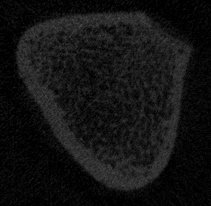
To quantify measures of trabecular bones, trabecular segmentation and analysis are performed. Figure 2A shows the setting dialog for trabecular segmentation, where trabecular bones in the selected region are segmented and extracted (Figure 2B), and segmentation results using the supplied parameters can be checked slice-by-slice visually. Subsequently, trabecular bones are analyzed with satisfactory parameters (Figure 3A). Depending on the selection statuses of reporting options, raw quantifications of bone volume (BV), total volume (TV), sum of gray values (Intensity), and thicknesses measured either two dimensionally or three dimensionally (Table 2) are reported. Finally, calibration information is extracted from the scanned micro-CT dataset and calibrated measures of BV, TV, BMC, BV/TV, and BMD are calculated followed by profiling their distributions in the selected analyzing region layer-by-layer against the layer positions (Figure 4).
As a quality-control feature of the plugin, quantification of simulated objects is supported. Simulated standard objects with known dimensions are quantified by the plugin for comparison with the theoretical values or measures from other software, such as commercial software supplied with micro-CT machines or BoneJ14, a free open source plugin for bone image analysis. For analyzing simulated objects, the noise settings are set to zero, as simulated images are considered high quality images without any noise. Objects with various thicknesses were simulated and results are shown (Figure 3, Table 3). For simulated standard 2D objects, such as circles, squares and rectangles, exact values for area (TV or BV) and thickness are reported (Table 3). For 3D objects, exact thickness measures for cubes, spheres, and cuboids are reported, however, the thicknesses for cylinders are not accurate for voxels near cylinder's both ends, while the voxel thicknesses in the middle slices of the cylinders are exactly as predicted. This is a feature of the underlying thickness measurement algorithm, wherein the voxel's thickness for each object is determined by the diameter of the largest sphere, or the side length of the largest cube, which contains this voxel and is completely inside the object. Therefore, thicknesses of objects made of different spheres and cubes can be measured accurately, while cylinders can only be measured accurately in the middle slice's radius-distance away from both ends.
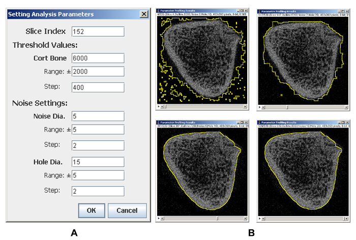
Figure 1: Representative results of parameter profiling analysis. (A) The parameters setting page. (B) Representative results of parameter profiling analysis. Some parameter combinations are better than others for detecting the outer boundaries of bones. Please click here to view a larger version of this figure.
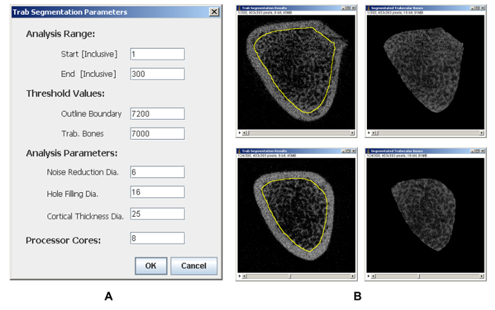
Figure 2: Representative results of trabecular segmentation analysis. (A) The parameters setting page. (B) Representative segmentation results of trabecular bones at different layers. Please click here to view a larger version of this figure.
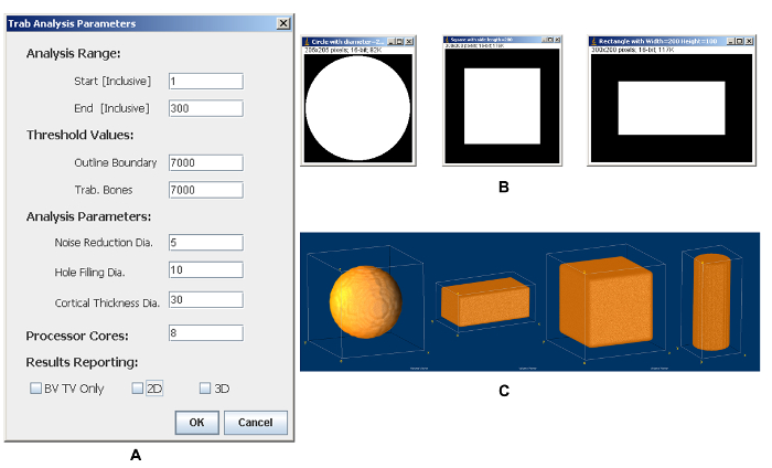
Figure 3: Trabecular analysis. (A) The parameters setting page. (B) Representative results of simulated 2D objects. (C) Representative results of simulated 3D objects visualized by 3D volume viewer. Please click here to view a larger version of this figure.
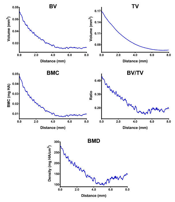
Figure 4: Distributions of trabecular bone measures in the selected analyzing region. The horizontal axis represents the relative distance to the starting slice layer in the analyzing region. Values in the Y-axis are calibrated trabecular measures in the analyzing region. Please click here to view a larger version of this figure.
Slice | Outline Boundary | Noise Reduction Dia. | Hole Filling Dia. |
4 | 5200 | 0 | 10 |
147 | 5200 | 2 | 20 |
361 | 7200 | 6 | 16 |
539 | 8000 | 10 | 20 |
Table 1: Representative results of parameter profiling analysis.
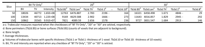
Table 2: Representative results of trabecular analysis.
Object | Dimension | Volumeb | Surfacec | Thickness |
Square | 200 X 200 | 40000 | 796 | 200 |
Rectangle | 200 X 100 | 20000 | 596 | 100 |
Circle | Dia: 200 | 31428 | 796 | 200 |
Cube | 30 X 30 X 30 | 27000 | 5048 | 30 |
Cuboid | 80 X 40 X 30 | 96000 | 13008 | 30 |
Sphere | Dia: 30 | 14328 | 3944 | 30 |
Cylinderd | Dia:30; H: 100 | 71600 | 12800 | 27.84 |
Cylindere | Dia:30; H: 100 | 51552 | 9552 | 30 |
a: Results are in raw voxels. Dia: diameter; H: height. | ||||
b: Volume (3D) or area (2D). | ||||
c: Surface (3D) or perimeter (2D). | ||||
d: Measurs from slice 1 to slice 100 are used for analysis. | ||||
e: Measurs from slice 15 to slice 85 are used for analysis. |
Table 3: Quantification results for simulated objects.
Supplementary File 1. Sample bone. Please click here to download this file.
This study describes an ImageJ plugin for analyzing trabecular bones, which is automatic, efficient, and user friendly. The plugin can also be used to quantify any 2D or 3D object for layer-by-layer measures of areas, volumes, and thicknesses. Currently, only a single measured value for each trabecular parameter is reported for each sample by standard micro-CT analysis, which cannot fully represent the characteristics of the measured entity in the selected analyzing region. The described plugin reports layer-by-layer quantities of each parameter for each sample, which fully retains the distribution information of the measured parameter in the selected analyzing region, and therefore more advanced and sensitive statistical approaches are applicable for analyzing such data.
With the standard, semi-automatic hand-contouring segmentation method, substantial variation between different hand-contouring slices were observed with operator bias8,9,10, warranting a more uniform and automatic method for trabecular segmentation. As the contrast is maximal between the scanning background and the bone outer boundary, outer-boundary assisted trabecular segmentation is performed by the plugin, where the bone's outer boundary can be automatically detected with accuracy when appropriate threshold, noise, and hole settings are provided. To facilitate the determination of segmentation parameters, a range of parameter combinations are profiled one by one using a representative slice from the analyzing region, and satisfactory segmentation results are checked visually. Subsequently, trabecular bones are analyzed with the profiled parameters. When appropriate segmentation parameters are set, and the plugin has been successfully applied to analyze trabecular bones from rat distal femurs treated with different bone anabolic agents5, reproducible results are reported for the same image without operator bias.
The plugin currently can only process one sample at a time. If multiple samples are present in the image, all samples are quantified as a single object without discrimination. Therefore, preprocessing is required if multiple samples are scanned simultaneously in a single sample tube. The quantification outputs are raw measures of pixel counts or gray values, which should be calibrated manually using appropriate calibration information.
The most critical step in this protocol is selecting appropriate parameters for trabecular analysis. Generally, groups of bone samples are analyzed using identical segmentation parameters to make the results comparable. In such a case, care should be taken to ensure that segmentation results for all samples are examined visually for potential errors before further analyses are conducted.
A major limitation of this technique is that the noise reduction settings are applied to cortical bones only for contouring a bone's outer boundary, but not on extracted trabecular bones. As various filtering strategies have been reported15 as optimal for trabecular analysis under different conditions, no single filter is good for all image samples. Therefore, there is no built-in filtration step before quantification of trabecular bones. To be compatible with the output by software with built-in image filtrations, extracted trabecular bones can be processed similarly first using various imaging tools, and then imported into ImageJ and quantified by the plugin subsequently. Moreover, different image formats are generated by different micro-CT vendors, and most of them cannot be imported or opened by ImageJ directly, thus modules for importing various image formats into ImageJ for further analysis are desired. Another limitation is that the 3D thicknesses in slices near the ends of the selection range are not accurate if part of the objects are outside of the selection range, which is also true for any available 3D quantification packages, therefore, a larger range of slices should be quantified, and only the middle portion of selected slices should be used for further analysis. Such an approach can only be available when measured quantities are reported layer-by-layer as shown in this plugin, but not for measurements that only a single value is reported for each quantified parameter in the selection range.
The authors have nothing to disclose.
This work was partially supported by grant NFSC 81170806. The authors would like to thank the micro-CT core facility of School of Stomatology, Wuhan University for helping scan and analyze the rat femurs.
ImageJ | NIH | imagej | Any version with a java 1.8 run time |
trabecular analysis plugin | Bomomics | bomomics | free or commercial version |
Micro CT scanner | Scanco | μ-50 | micro CT from any vendor |
Computer System | Lenovo | any brand | |
Windows Operating System | Microsoft | Windows 7 x64 | any 64-bit Windows operating system |
Office Software | Microsoft | Office 2010 | any speadsheet software that has xy chart function |