All procedures described were approved by the Drexel University Institutional Animal Care and Use Committee (IACUC). The neonatal piglet was acquired from a United States Department of Agriculture (USDA)-approved farm located in Pennsylvania, USA.
1. Stereo-imaging system setup
- Attach a stereo-imaging camera system that captures up to 100 frames/s (FPS) to a utility stand. The stereo-imaging camera system used in this study is a passive stereo camera with two horizontally aligned cameras (referred to as the left and right cameras) separated by a baseline of 63 mm (Figure 1).
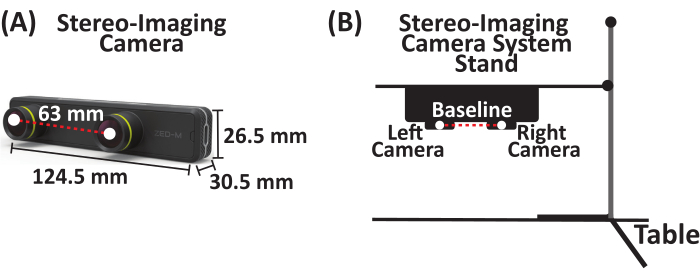
Figure 1: Stereo-imaging camera system. (A) Parallel stereo-imaging camera system with two cameras (left and right cameras) separated by a baseline of 63 mm. (B) Schematic of stereo-imaging camera system and stand setup. Please click here to view a larger version of this figure.
2. Stereo-imaging system DLT Calibration-digitizing the 3D control volume
- Obtain three clear acrylic plexiglass square sheets (12 in x 12 in x 0.125 in). On each sheet, place a grid and draw at least 10 points, resulting in a minimum of 30 points distributed across the 3D control volume in the x, y, and z coordinate planes. Construct the 3D control volume by stacking the three sheets at varying heights to capture the maximum height of what will be recorded (Figure 2A).
- Digitize all the points on the 3D control volume using a digitizer with a foot pedal. Acquire x, y, and z coordinates (in mm) (Figure 2B) by establishing the origin (0, 0, 0) on the 3D control cube, defining the positive x- and y-directions, opening a document to save the digitized (x, y, z) coordinates (in mm) of each point, and saving (x, y, z) coordinates (in mm) as a *.csv file.
NOTE: The (x, y, z) coordinates are relative to the set origin on the 3D control cube. - Use these digitized (x, y, z) coordinates (in mm) to calibrate the stereo-imaging camera system's left and right cameras, respectively.
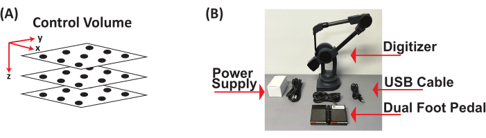
Figure 2: Three-dimensional control volume and digitizer with foot pedal. (A) Schematic of 3D control volume. (B) Components of digitizer with foot pedal used to digitize 3D control volume to obtain (x, y, z) coordinates in mm. Abbreviation: 3D = three-dimensional. Please click here to view a larger version of this figure.
3. Stereo-imaging camera system calibration-generation of direct linear transformation coefficients
- Attach the stereo-imaging camera system to a utility stand (Figure 3A).
- Position the stereo-imaging camera system 6 cm above the 3D control volume (Figure 3A).
- Connect the stereo-imaging camera system to a laptop via a USB type-C cable.
- Open the imaging software (see the Table of Materials).
- Image the 3D control volume. The output image (Supplemental Figure S1) includes both the left and right camera views (Figure 3B).
- Run the custom MATLAB code (Supplemental File 1) to separate the output image into two images, left and right images, respectively (Figure 3C, Supplemental Figures S2, and Supplemental Figures S3, respectively).
- Click Run to initialize the DLTcal5.m GUI22 (Supplemental File 2).
- Click initialize on the DLTcal5 controls window to select the *.csv file with the digitized (x, y, z) coordinates (in mm) (Figure 4A and Supplemental File 3).
- Select the corresponding image of the 3D control volume from the first view of the stereo-imaging camera system (Supplemental Figure S2). For this stereo-imaging camera system, the left camera view corresponds to the first camera view (Figure 4B).
- The first camera view image (i.e., left camera view) pops up.
- Select the points in the order the points were digitized in Section 2 to obtain the 2D pixel coordinates from the left camera view (Figure 4B).
- Set current point on the DLTcal5 Controls window and click on the corresponding current point on the loaded first camera view (i.e., left camera view) image.
- After selecting all the points on the loaded first camera view, click compute coefficients to generate the 11 DLT coefficients for the left camera view (Figure 4B).
- Click add a camera on the DLTcal5 controls window and repeat steps 3.7.2-3.7.6 to generate the 11 DLT coefficients for the right camera view (i.e., second camera view) (Figure 4B, C and Supplemental Figure S3).
- Click save data on the DLTcal5 controls window to select the folder where the output files will be saved (Figure 4D).
- The output files include the 2D (x, y) pixel coordinates (Supplemental File 4) and corresponding 11 DLT coefficients for the left and right camera views of the stereo-imaging camera system (Figure 4D and Supplemental File 5).
- The stereo-imaging camera system is calibrated.
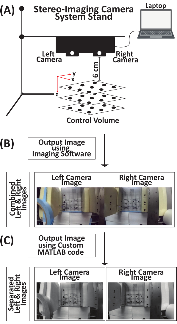
Figure 3: Schematic for acquiring an image of three-dimensional control volume using a stereo-imaging camera system for direct linear transformation calibration. (A) Attach the stereo-imaging camera system to a stand and then connect it to a laptop via a USB type-C cable. Place the 3D control volume 6 cm under the stereo-imaging camera system. (B) Using the imaging software, take an image of the 3D control volume. The output image is a combined image from the left and right cameras. (C) Using a custom MATLAB code, the combined output image is separated into individual left and right images of the 3D control volume. Abbreviation: 3D = three-dimensional. Please click here to view a larger version of this figure.
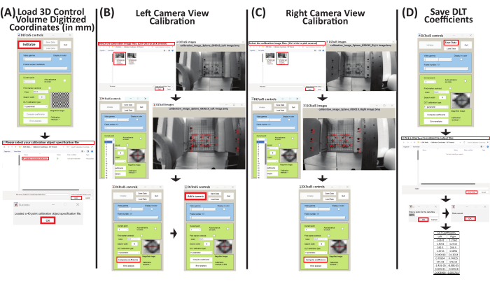
Figure 4: Schematic for generating direct linear transformation coefficients for left and right camera views of a stereo-camera imaging system. (A) Run DLTcal5.m22, click initialize on the controls window, and select the *.csv file with the digitized (x, y, z) coordinates (in mm) of the 3D control volume. (B) Select the calibration image of the left camera view. Then, select the points on the image in the same order that they were digitized. Then, click compute coefficients to generate the DLT coefficients for the left camera view. Next, click Add camera to repeat the steps for the right camera view. (C) Select the calibration image of the right camera view. Then, select the points on the image in the same order that they were digitized. Then, click compute coefficients to generate the DLT coefficients for the right camera view. (D) Click Save Data to select the directory to save the DLT coefficients for the left and right camera views. Enter the name for the output file and click OK and the DLT coefficients are saved as a *.csv file. Abbreviation: 3D = three-dimensional and DLT = direct linear transformation. Please click here to view a larger version of this figure.
4. Data acquisition
- Place anesthetized neonatal Yorkshire piglet (3-5 days old) in a supine position with upper limbs in abduction to expose the axillary region. Make a midline incision through the skin and fascia overlying the trachea down to the upper third of the sternum.
- Use blunt dissection to expose the brachial plexus nerves.
- Squirt saline solution on the exposed brachial plexus nerve to keep them hydrated before, during, and after testing.
- Cut the distal end of a brachial plexus PN and clamp to the mechanical testing apparatus.
- Attach the stereo-imaging camera system to the utility stand, place it up to 6 cm above the PN to be stretched, and then connect the stereo-imaging camera system to a laptop via a USB type-C cable (Figure 5A).
- Use an ink-based skin marker to place markers on the insertion and clamp sites and an additional two to four markers along the length of the PN depending on the nerve length, for displacement tracking (Figure 5B).
- Place a calibration grid (i.e., laminated grid with 0.5 cm x 0.5 cm squares) and a 1 cm ruler, flat underneath the PN for data analysis (Figure 5B).
- Record the initial length of the PN after clamping and just before stretching.
- Stretch the PN at a displacement rate of 500 mm/min to failure or a predetermined stretch.
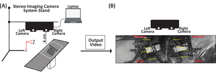
Figure 5: Representative schematic for data acquisition of peripheral nerve stretching. (A) Attach the stereo-imaging camera system to a stand and then connect it to a laptop via a USB type-C cable. Place the stereo-imaging camera system up to 6 cm above the peripheral nerve. (B) The peripheral nerve is clamped to the mechanical setup at the distal end. Using an ink-based skin marker, place a marker on the insertion and clamp sites and an additional two to four markers along the nerve length. Saline is squirted on the peripheral nerve to keep it hydrated before, during, and after testing. Please click here to view a larger version of this figure.
5. Data analysis-marker trajectory tracking
- Run the custom MATLAB code (Supplemental File 6) to separate the output video file (Supplemental File 7) into two video files, left and right camera video files (Supplemental File 8 and Supplemental File 9, respectively).
- Click Run to initialize the DLTdv7.m22 GUI (Supplemental File 10).
- The DLTdv7 controls window pops up and the new project, load project, and quit buttons are enabled (Figure 6A).
- Click new project on the DLTdv7 controls window to begin a new project.
- When a dialog box pops up, select 2 to indicate two video files (i.e., left and right camera views) to track the displacement marker trajectories on a stretched peripheral nerve (Figure 6B).
- Select the first video file (i.e., Video 1), which is the video file from the left camera view (Supplemental File 8), and click open (Figure 6C). Then, select the second video file (i.e., Video 2), which is the video file from the right camera view (Supplemental File 9), and click open (Figure 6C).
- After the two video files are selected, click yes to signify the video files were acquired from camera views calibrated via DLT.
- Select the corresponding DLT coefficients *.csv file (Supplemental File 5) for the stereo-imaging camera system and click on open (Figure 6D).
- The initial video frames are displayed from both video files and the rest of the DLTdv7 controls window is activated. The new project button is replaced with the recompute 3D points button and the load project button is replaced with the save button (Figure 6E).
- On the DLTdv7 controls window, ensure the frame number is on 1, the current point is set to 1, autotrack mode is off, and update all videos, DLT visual feedback, and show 2D tracks are checked (Figure 6E).
- Ensure that the tracking points are placed on the displacement markers of the PN such that the insertion marker corresponds to point 1, marker 1 corresponds to point 2, and so on with the clamp marker being the final point.
- Place point 1 on the insertion marker on Video 1 (i.e., left camera view video file) ensuring the placed point is at the center of the insertion marker. Use keyboard shortcuts (Table 1) to move the placed point to the center of the insertion marker (Figure 7A).
- Because DLT visual feedback is checked, when a point is placed in Video 1, a blue epipolar line appears in Video 2 (i.e., right camera view video file) (Figure 7). Place point 1 on the insertion marker in Video 2 using the blue epipolar line as reference. Use the keyboard shortcuts (Table 1), as needed, to move the placed point to the center of the insertion marker (Figure 7A).
- Click add a point on the DLTdv7 controls window to add points on the other tissue markers to track their trajectories. Refer to the current point on the DLTdv7 controls window to know which point is active.
- Click add a point. Place point 2 on marker 1 de Video 1. Use the blue epipolar line and keyboard shortcuts to place point 2 on marker 1 de Video 2. Continue adding and placing points, first on Video 1 and then on Video 2, for all displacement markers along the length of the nerve between the insertion and clamp (i.e., final point) (Figure 7B-F).
- Once all initial points are placed in Video 1 and Video 2 (i.e., the left and right camera video files, respectively), ensure the frame number is on 1 and the current point is set to 1 on the DLTdv7 controls window.
- On the DLTdv7 controls window, change autotrack mode à auto-advance from the dropdown menu and autotrack predictor à extended Kalman from the dropdown menu (Figure 8A).
- Complete the tracking of all the placed points in Video 1 first and then complete tracking in Video 2. Track the marker trajectory by left-clicking on the center of the marker frame by frame until failure (i.e., frame before gross rupture of the peripheral nerve) or the entirety of the video for predetermined stretch is achieved.
- Begin tracking point 1 de Video 1. Zoom in and out (Table 1) as desired to ensure tracking is at the center of the marker; click frame by frame until the failure or end of the video (Figure 8B). After completing the tracking of point 1 de Video 1, return to frame 1 and change the current point to point 2 from the dropdown menu on the DLTdv7 controls window. The previous tracked point will turn light blue and its trajectory will turn yellow. The current point will have a green diamond and a pink center.
- Complete the tracking of all the points in Video 1 by left-clicking frame by frame for each point until failure or end of the video (Figure 8C-G).
- In Video 2, use the blue epipolar line to track points in reference to Video 1 (Figure 9). On the DLTdv7 controls window, return frame number à 1 and set current point à 1, and begin tracking point 1's trajectory in Video 2.
- Follow the same steps (5.2.16-5.2.18) to track the remaining points in Video 2.
- After tracking is complete in Video 1 and Video 2, click export points on the DLTdv7 controls window to export the (x, y, z) coordinates (in mm) of the tracked points.
- A dialog box pops up to select the directory where to save the output files. Click on the directory location.
- Another dialog box pops up to set the name of the output files. Set the output files' name (i.e., nerve1_101-Jan-2001videoanalyzed_cal09.30_trial1_).
- Another dialogue box pops up. Select the save format as flat.
- Another dialog box pops up. Select no to calculate the 95% confidence interval.
- A final dialog box pops up that shows the data is exported and saved, and the four output files are exported to the selected directory location (Supplemental File 11, Supplemental File 12, Supplemental File 13, and Supplemental File 14).
- Click save project on the DLTdv7 controls window to save the current project (Supplemental File 15) in the same directory as the output files.
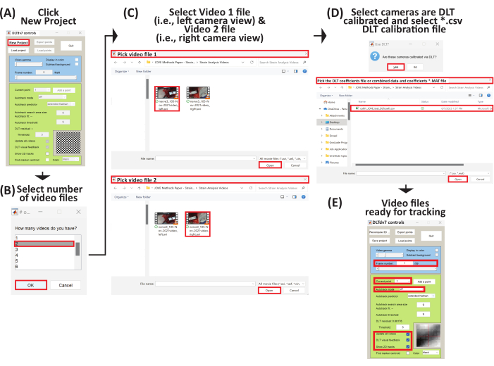
Figure 6: Schematic to set up a new project to begin three-dimensional trajectory tracking. (A) Run DLTdv7.m22 and click New Project to begin a new project. (B) Select 2 as the number of video files. (C) Select Video 1 file (i.e., left camera view) and then select Video 2 file (i.e., right camera view). (D) Select yes as the video files come from a DLT calibrated stereo-imaging camera system. Then, select the *.csv file containing the DLT coefficients. (E) The selected video files are now ready for tracking. Please click here to view a larger version of this figure.
| Key/Click | Description |
| Left Click | Tracks trajecgtory of a point in frame clicked |
| (+) Key | Zooms current video frame de arount mosue pointer |
| (-) Key | Zooms current video frame out arount mosue pointer |
| (i) Key | Move point up |
| (j) Key | Move point left |
| (k) Key | Move point right |
| (m) Key | Move point down |
Table 1: Keyboard and mouse shortcuts for tracking point trajectory.
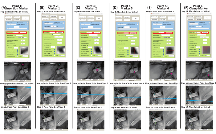
Figure 7: Schematic to place initial points on tissue markers for Video 1 and Video 2 using DLTdv7.m22. (A) Set current point à 1. Place point 1 on the insertion marker de Video 1. Using the blue epipolar line in Video 2, place point 1 on the insertion marker. (B) Set current point à 2. Place point 2 on marker 1 de Video 1. Using the blue epipolar line in Video 2, place point 2 on marker 1. (C) Set current point à 3. Place point 3 on marker 2 de Video 1. Using the blue epipolar line in Video 2, place point 3 on marker 2. (D) Set current point à 4. Place point 4 on marker 3 de Video 1. Using the blue epipolar line in Video 2, place point 4 on marker 3. (E) Set current point à 5. Place point 5 on marker 4 de Video 1. Using the blue epipolar line in Video 2, place point 5 on marker 4. (F) Set current point à 6. Place point 6 on the clamp marker de Video 1. Using the blue epipolar line in Video 2, place point 6 on the clamp marker. Please click here to view a larger version of this figure.
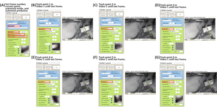
Figure 8: Schematic for tracking marker point trajectories of Video 1 using DLTdv7.m22. (A) Set frame number à 1, current point à 1, autotrack mode à auto-advance, and autotrack predictor à extended Kalman. (B) Set current point à 1. On Video 1 file, begin tracking the insertion marker (i.e., point 1) displacement by left-clicking frame-by-frame until the last frame. (C) Set frame number à 1 and current point à 2. On Video 1 file, begin tracking marker 1 (i.e., point 2) displacement by left-clicking frame-by-frame until the last frame. (D) Set frame number à 1 and current point à 3. On Video 1 file, begin tracking marker 2 (i.e., point 3) displacement by left-clicking frame-by-frame until the last frame. (E) Set frame number à 1 and current point à 4. On Video 1 file, begin tracking marker 3 (i.e., point 4) displacement by left-clicking frame-by-frame until the last frame. (F) Set frame number à 1 and current point à 5. On Video 1 file, begin tracking marker 4 (i.e., point 5) displacement by left-clicking frame-by-frame until the last frame. (G) Set frame number à 1 and current point à 6. On Video 1 file, begin tracking the clamp marker (i.e., point 6) displacement by left-clicking frame-by-frame until the last frame. Please click here to view a larger version of this figure.
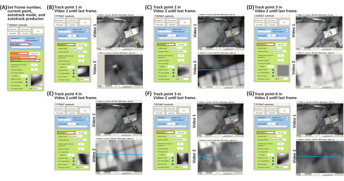
Figure 9: Schematic for tracking marker point trajectories of Video 2 using DLTdv7.m22. (A) Set frame number à 1, current point à 1, autotrack mode à auto-advance, and autotrack predictor à extended Kalman. (B) Set current point à 1. Using the blue epipolar line on Video 2 file, begin tracking the insertion marker (i.e., point 1) displacement by left-clicking frame-by-frame until the last frame. (C) Set frame number à 1 and current point à 2. Using the blue epipolar line on Video 2 file, begin tracking marker 1 (i.e., point 2) displacement by left-clicking frame-by-frame until the last frame. (D) Set frame number à 1 and current point à 3. Using the blue epipolar line on Video 2 file, begin tracking marker 2 (i.e., point 3) displacement by left-clicking frame-by-frame until the last frame. (E) Set frame number à 1 and current point à 4. Using the blue epipolar line on Video 2 file, begin tracking marker 3 (i.e., point 4) displacement by left-clicking frame-by-frame until the last frame. (F) Set frame number à 1 and current point à 5. Using the blue epipolar line on Video 2 file, begin tracking marker 4 (i.e., point 5) displacement by left-clicking frame-by-frame until the last frame. (G) Set frame number à 1 and current point à 6. Using the blue epipolar line on Video 2 file, begin tracking the clamp marker (i.e., point 6) displacement by left-clicking frame-by-frame until the last frame. Please click here to view a larger version of this figure.
6. Data analysis-strain analysis
- Run a custom MATLAB code (Supplemental File 16) to import the tracked 3D (x, y, z) marker trajectories (in mm).
- On the MATLAB command window, type:
percentStrain, deltaLi, lengthNi, filename] = PercentStrain_3D - Enter the rupture time, for example, if the video files have 59 frames, the time is 0.59 s; enter the number of tracked points, and select the *_xyzpts.csv file, with the tracked 3D (x, y, z) trajectories (in mm).
- Select the directory to save the output length vs time (Supplemental Figure S4), change in length vs time (Supplemental Figure S5), and strain vs time (Supplemental Figure S6) plots and *.xls file with time, length, change in length, and strain (Supplemental File 17).
- Calculate the length (l), change in length (Δl), and percent strain using equations 1-3:
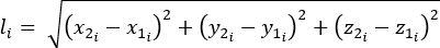 (1)
(1)
Where li is the distance between any two markers at any time point; x1i, y1i, z1i are the 3D coordinates of one of the two markers; and x2i, y2i, z2i are the 3D coordinates of the second markers.
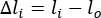 (2)
(2)
Where li is the distance between any two markers at any time point, and lo is the distance between any two markers at the original/zero-time point.
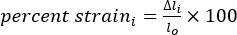 (3)
(3)
Where Δli is the change in length between two markers at any time point, and lo is the distance between any two markers at the original/zero-time point.
Using the described methodology, various output files are obtained. The DLTdv7.m *_xyzpts.csv (Supplemental File 12) contains the (x, y, z) coordinates in millimeters of each tracked point at each time frame that is further used to calculate the length, change in length, and strain of the stretched PN. Representative length-time, change in length-time, and strain-time plots of a stretched PN are shown in Figure 10. The stretched PN had an insertion marker, four markers along its length, and a clamp marker comprising six segments. By quantifying the overall and segmental strains of the stretched PN, a better understanding is gained of the non-homogeneity of these structures as well as the segmental contribution to the overall stretch. The length-time (Figure 10A) and change in length-time plots (Figure 10B) are used to calculate the strain-time plots (Figure 10C). In addition to the plots, a spreadsheet (Supplemental File 17) with the plot data (i.e., time, length, change in length, and strain) is exported.
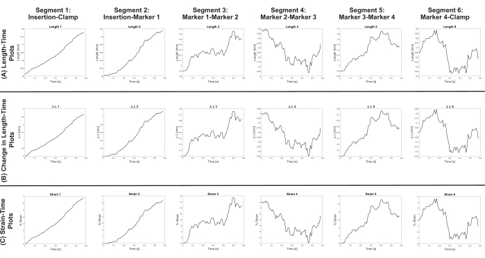
Figure 10: Representative plots of strain-time, change in length-time, and length-time of a stretched peripheral nerve. (A) Length-time plots of the entire nerve (i.e., segment 1) and for all segments between adjacent markers (i.e., segments 2-6). (B) Change in length-time plots of the entire nerve (i.e., segment 1) and for all segments between adjacent markers (i.e., segments 2-6). (C) Strain-time plots of the entire nerve (i.e., segment 1) and for all segments between adjacent markers (i.e., segments 2-6). Please click here to view a larger version of this figure.
The other three DLTdv7.m output files (Supplemental File 11, Supplemental File 13, and Supplemental File 14) and output project (Supplemental File 15) are used to reload the project in case the marker points' trajectories need to be retracked.
Supplemental Figure S1: Output image of three-dimensional (3D) control volume. Output image of 3D control volume taken using the parallel stereo-imaging camera system and imaging software system for direct linear transformation calibration. Please click here to download this File.
Supplemental Figure S2: Left image of three-dimensional (3D) control volume. Left image of 3D control volume used for direct linear transformation calibration. Please click here to download this File.
Supplemental Figure S3: Right image of three-dimensional (3D) control volume. Right image of 3D control volume used for direct linear transformation calibration. Please click here to download this File.
Supplemental Figure S4: Length-time output plots. (A–F) Length-time output plots of each segment at each time frame. Please click here to download this File.
Supplemental Figure S5: Change in length-time output plots. (A–F) Change in length-time output plots of each segment at each time frame. Please click here to download this File.
Supplemental Figure S6: Strain-time output plots. (A–F) Length-time output plots of each segment at each time frame. Please click here to download this File.
Supplemental File 1: Custom MATLAB code crop_left_right_stereoimage.m. Custom MATLAB code used to separate the output image into two images, left and right images, respectively. Please click here to download this File.
Supplemental File 2: DLTcal5.m22. Open-source MATLAB code used to obtain the direct linear transformation coefficients of the parallel stereo-imaging camera system. Please click here to download this File.
Supplemental File 3: Three-dimensional (3D) Control Volume Digitized Points. Spreadsheet file (3D Control Volume_Digitized Pts.csv) containing the digitized (x, y, z) points in millimeters of the points on the 3D control volume. Please click here to download this File.
Supplemental File 4: DLTcal5.m output spreadsheet file containing the (x, y) pixel coordinates of the three-dimensional (3D) control volume points. Output spreadsheet file (cal01_JOVE_test_xypts.csv) containing the (x, y) pixel coordinates of the 3D control volume points using DLTcal5.m22. Please click here to download this File.
Supplemental File 5: DLTcal5.m output spreadsheet file containing the 11 direct linear transformation (DLT) coefficients. Output spreadsheet file (cal01_JOVE_test_DLTcoefs.csv) containing the 11 DLT coefficients for the left and right camera views of the stereo-imaging camera system using DLTcal5.m22. Please click here to download this File.
Supplemental File 6: Custom MATLAB code crop_left_right_stereovideo.m. Custom MATLAB code used to separate the output video file into two video files, left and right camera video files. Please click here to download this File.
Supplemental File 7: Output video file of a stretched peripheral nerve. Output video file (nerve3_105-Nov-2021video.avi) of a stretched peripheral nerve containing the combined video files of the left and right camera views. Please click here to download this File.
Supplemental File 8: Left camera view video file (i.e., Video 1) of a stretched peripheral nerve. Left camera view video file (nerve3_105-Nov-2021video_left.avi) of a stretched peripheral nerve used to track marker point trajectories using DLTdv7.m22. Please click here to download this File.
Supplemental File 9: Right camera view video file (i.e., Video 2) of a stretched peripheral nerve. Right camera view video file (nerve3_105-Nov-2021video_right.avi) of a stretched peripheral nerve used to track maker point trajectories using DLTdv.7.m22. Please click here to download this File.
Supplemental File 10: DLTdv7.m22. Open source MATLAB code used to track marker point trajectories of video files obtained from a stereo-imaging camera system calibrated using direct linear transformation. Please click here to download this File.
Supplemental File 11: DLTdv7.m output file *_xypts.csv. The first DLTdv7.m output file is *_xypts.csv (nerve3_105-Nov-2021videoanalyzed_cal09.30_trial1_xypts.csv) contains the pixel coordinates (x1, y1), (x2, y2), etc…for each tracked point at each time frame. Please click here to download this File.
Supplemental File 12: DLTdv7.m output file *_xyzpts.csv. The second DLTdv7.m output file is *_xyzpts.csv (nerve3_105-Nov-2021videoanalyzed_cal09.30_trial1_xyzpts.csv) contains the real-world coordinates in millimeters (x1, y1, z1), (x2, y2, z2), etc…for each tracked point at each time frame. Please click here to download this File.
Supplemental File 13: DLTdv7.m output file *_xyzres.csv. The third DLTdv7.m output file is *_xyzres.csv (nerve3_105-Nov-2021videoanalyzed_cal09.30_trial1_xyzres.csv) contains the DLT residual for each tracked point at each time frame. Please click here to download this File.
Supplemental File 14: DLTdv7.m output file *_offset.csv. The first DLTdv7.m output file is *_offset.csv (nerve3_105-Nov-2021videoanalyzed_cal09.30_trial1_offsets.csv) contains video 1 and video 2 offset for each tracked point at each time frame. Please click here to download this File.
Supplemental File 15: DLTdv7.m project output file *_dvProject.mat. The DLTdv7.m project output file (nerve3_105-Nov-2021videoanalyzed_cal09.30_trial1_dvProject.mat) contains the paths of the video files, all interface settings, all clicked marker point trajectories, and calibration information allowing for easy reload of project to make changes, if necessary. Please click here to download this File.
Supplemental File 16: Custom MATLAB code PercentStrain_3D.m. Custom MATLAB code used to calculate length, change in length, and percent strain of a stretched nerve between adjacent markers at each time point. Please click here to download this File.
Supplement File 17: PrecentStrain_3D.m output file *_3Dstrain.xls. Output file *_3Dstrain.xls (nerve3_105-Nov-2021_3Dstrain.xls) that contains time, length, change in length, and strain of each tracked point at each time frame. Please click here to download this File.
