In order to determine the Pf and compare the activity of different AQPs, mesophyll protoplasts from Arabidopsis leaf are used. These protoplasts were found to have low basal (background) Pf levels 7 and can serve as a functional-expression system to enable reproducible Pf measurements.
Protoplasts from a mature leaf from a 6 week old Arabidopsis plant were isolated and three gene constructs with AQP genes from Arabidopsis (AtPIP2;1) and maize (ZmPIP1;2 and ZmPIP2;4) were transiently (and separately) expressed using the PEG transformation method 15. Assuming that the event of transformation is simultaneous for a large number of plasmids applied to the cell irrespective of their nature and based on the results which showed a 100% success rate for synchronized transient expression of two plasmids in one cell reported previously for other plant systems 15,16, they were co-transformed with a vector encoding the enhanced green fluorescent protein (eGFP) in order to label the transformed protoplasts (Figure 7).
For the Pf assays, protoplasts were set in the experimental chamber (Figure 1B) and the GFP labeled protoplasts were monitored by video while they were flushed initially with the isotonic solution (600 mOsm), then with the hypotonic solution (500 mOsm), using the perfusion system (Figure 1A).
The time courses of the cell volume changes (Figure 8A) were obtained for each cell in two stages: first, the ‘Image Explorer’ and ‘Protoplast Analyzer’ plugins were used to generate the time course of changes in the cell contour area (Figure 2), then, the Matlab fitting program PfFit (Figure 5) was used to import these areas and convert them to cell volumes. The Pf values (Figure 8C) were derived for each cell using the PfFit program (Figure 5), based on the time course of the cell volumes and, additionally, on the imported averaged time course of the transmittance changes of the Indicator Dye (Figure 3), converted to the time course of the Indicator Dye concentration change (Figure 4A) and then – to the time course of the bath osmolarity change (Figures 4B, 6A and 8B). It is worth noting, that delC, the difference in osmotic concentrations in the cell (Cin) and in the bath (Cout), i.e., the driving force for the water influx, was due almost only to the change of Cout (Figure 6A). In this experiment, Pf increased during the assay (Figure 6B).
The Pf values of the protoplasts transformed with each of the three AQPs were significantly higher than the Pf of the control cell transformed with GFP alone (Figure 8C).
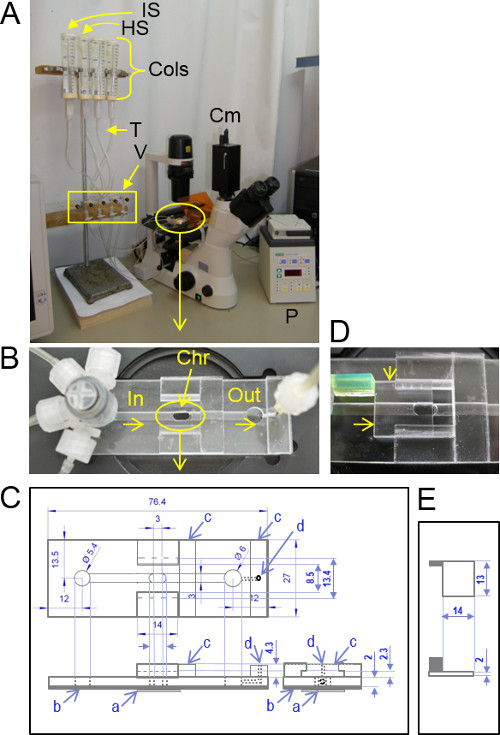
Figure 1: The volume-assay system. (A) The experimental setup: The perfusion system contains solution reservoirs (infusion columns, ‘Cols’), tubing (T), valves (V) and a peristaltic pump (P) connected to the plexiglass slide set on the microscope table. HS = hypotonic solution, IS isotonic solution, Cm camera. (B) An enlarged view of the plexiglass slide with the experimental chamber (Chr) and the tubing attached via an inlet (In) manifold connector. The solution is sucked from the chamber via an outlet (Out) to the pump. (C) A schematic drawing of the plexiglass slide (counterclockwise: top view, long-side view and short-side view): a = glass cover slip, the central chamber bottom; b = clear adhesive tape (Table 1), serving as a bottom for the inlet and outlet solution grooves leading to and from the central chamber; when the Scotch tape is replaced (only occasionally), a hole is cut in it under the chamber; c = a plexiglass block glued to the slide; d = an outlet connector hole. Numbers are mm (but the drawing is not to scale). (D) An enlarged view of the center portion of the slide with the transparent cover (also plexiglass) partially covering the central chamber (arrows). (E) Schematic drawing (top and side views) of the transparent cover. The size of the transparent cover handle (green plastic in D) is arbitrary. Other details are as in C.

Figure 2: Analysis of swelling protoplasts images using the ‘Protoplast Analyzer’ plugin. (A) a, the first image of the movie with protoplasts, b, as in a, but yellow circles indicate the selection made after reviewing the movie, before the contours are autodetected, c, from the first till the last image the green circles tightly follow the contours of the “well-behaved” protoplasts undergoing analysis. (B) ‘Time’-course plots (with units of image number on the abscissa) of the calculated areas within the protoplast contours (‘Area’, in square pixels), for each tracked (and numbered) protoplast. (C) The parameters input panel of the ‘Protoplast analyzer’ plugin. Four ‘detection parameters’ can be adjusted to fine tune the protoplast detection algorithm. The ‘number of border pixels’ parameter sets the minimum thickness of the protoplast contour (default value: 5). The ‘relative weight’ parameter influences the grey level threshold difference between the inner protoplast area and the outer border (default: 2). The ‘maximum circumference ratio’ defines a threshold for excluding protoplasts whenever their shape deviates from a circle. This parameter is the ratio of the protoplast circumference to the circumference of a perfect circle having the same area as the protoplast (default: 1.05). The ‘maximum area increase’ (% increase per time step) parameter excludes protoplasts with contour area increases above the parameter value (default value: 5%). Finally, the plugin also handles small protoplast movements but will stop tracking protoplasts that move rapidly or that disappear from the image area. The movie can be rerun as many times as necessary, and a single protoplast can be reanalyzed separately. Please click here to view a larger version of this figure.
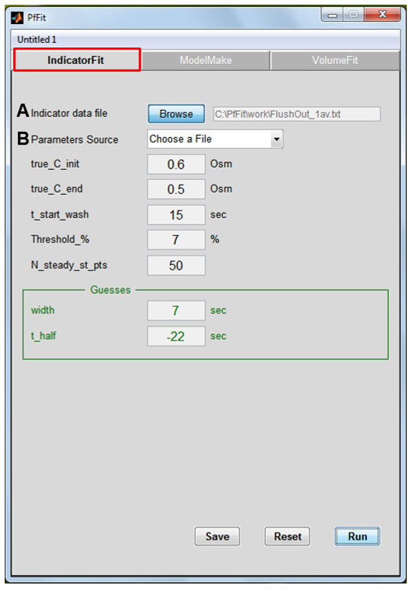
Figure 3: The ‘Indicator Fit’ panel of the PfFit program. This part translates the indicator transmittance time course into bath osmolarity time course. (A) Browse for the saved data file containing the time course of transmittance changes of the Indicator Dye. (B) Either use the previously saved list of variables and parameters, or insert manually the 5 variable values of the current experiment: ‘true_C_init’ and ‘true_C_end’ (the osmolarities of the initial bath solution and the Pf-assay solution perfused via the bath), ‘t_start_wash’ (the duration of baseline sampling at the initial Indicator Dye level), ‘threshold_%’ (% of baseline value, at which the program detects automatically the departure from baseline transmittance; 1 – 5% are usually the most effective), ‘N_steady_st_pts’ (the number of samples – with 10 samples representing every Indicator Dye image taken – to be averaged at the end steady state level of the Indicator Dye, crucial for the conversion of the Indicator Dye concentration to the osmoticum concentration) and initial guesses for two of the four parameters of the Indicator Dye transmittance sigmoidal time course, ‘width’ and thalf (roughly related to the duration of the transition part of the sigmoid, and to its midpoint, respectively; thalf may be negative!). Two best fit parameters, in addition to ‘width’ and thalf are obtained without the need for initial guesses: lag (‘flush_lag’), the time between the valve opening to the arrival of the solution in the bath, and ‘C_init’, without a physical meaning, but necessary for the description of the osmolarity time course (see the Supplemental PfFit User Guide.
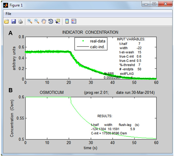
Figure 4: The Indicator Dye concentration in the bath and the osmolarity of the medium. (A) The time course of the Indicator Dye concentration, calculated directly from data (dots) and from the best-fit parameters (line) as it is washed away by a non dyed solution. (B) The calculated time course of the osmolarity change of the bath solution, assuming it follows the same dynamics as the change of the Indicator Dye concentration.
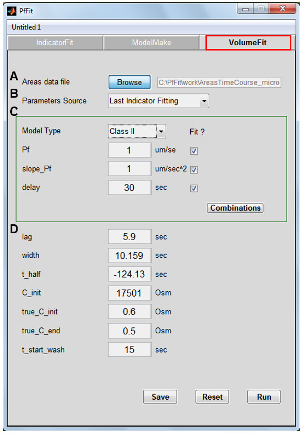
Figure 5: The ‘Volume Fit’ panel of the PfFit program. (A) Browse for the area time course data file of the analyzed protoplast. (B) Choose the ‘Last Indicator Fitting’ option to import the experiment parameters from the last run through the ‘Indicator Fit’ (see the Supplemental PfFit User Guide for alternatives). (C) ‘Model Type’ / ‘Class’: Class I contains the simplest model 1, Class II – models 2 – 5, class III – models 6 – 8. The models differ with respect to which parameters are being fixed and which are being adjusted (i.e., freely variable) during the fitting procedure (tick the box to allow it to vary), and whether or not ‘SlopePf’ and/or ‘Delay’ are null. The models 1 – 6 are discussed at length by Moshelion et al.11. ‘Combinations’ lists the parameter choices dictated by the choice of ‘Model Type’/‘Class’. Among models with a similar fit result – choose the simplest! Initialize the ‘Pf’, ‘SlopePf’ (‘Slope_Pf’) and ‘Delay’ parameters as shown (more details about ‘Delay’ in E below). (D) The variables and parameters describing the time course of the changing bath osmoticum are input either manually, or as described in B. (E) An interim plot, invoked by hitting ‘RUN’, of a time course of volume change (calculated from the cell contour areas) to aid in the choice of the initial value for the ‘Delay’ parameter. Estimate, by eyeballing, the total length of the baseline from the 1st point till the start of cell volume change (the ‘inclusive delay: the sum of ‘t-start-wash’ + ‘lag’/‘flush-lag’ + the “physiological” ‘delay’). Insert this value as an input parameter for the ‘delay’ in the ‘VolumeFit’ panel and ‘Run’ again (see also the Supplemental PfFit User Guide).
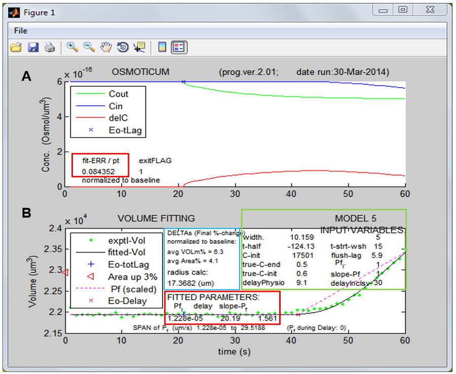
Figure 6: The results of fitting. (A) “Behind the scenes”: the calculated ultimate time courses of the osmoticum concentrations in the two compartments: the bath (Cout, green line) and the cell (Cin, blue line; Cin is calculated based on the protoplast volume change and an assumption that the plasma membrane is permeable only to water – the “perfect and true osmometer”11), and the time course of the difference between them (delC, red line), which is the driving force for water flow, ‘Eo-tLag’ marks the end of the ‘flush-lag’ and the start of the hypotonic challenge (here only at about 21 sec). Red box: the error of the fit value (fit-ERR, see definition in B below). (B) The ultimate result of fitting the volume time course; Green box: ‘INPUT VARIABLES’ are the values entered via the PfFit/‘VolumeFit’ panel (defined in Figure 5A legend). Black box: ‘exptl-Vol’ and ‘fitted-Vol’ are the experimental data and the volume calculated using the best-fit parameters, respectively, ‘Eo-tLag’ is the same as in A, ‘Eo-Delay’ marks the the start of volume change. ‘Area up 3%’ marks the volume at which the surface area increased by 3%, the presumed limit to the cell membrane ability to stretch without rupturing. ‘Pf (scaled)’ is the time course of the fitting-based calculated Pf, spanning the values indicated below the red box as ‘Span of Pf’. Red box: ’FITTED PARAMETERS’ are the values of the best fit parameters: ‘Pfi’ (the initial Pf), ‘delay’ (the period between the onset of the hypotonic challenge and the start of the volume change (which, according to the model 5 used in this example, is also the start in a change in the Pf value), and ‘slope-Pf’ (the constant rate of change in the Pf value. ‘fit_ERR’ shown in A – the minimization target of the Matlab fitting procedure – is the “root-mean-square” deviation (i.e., a square root of an averaged squared deviation) of a green dot from the black line), presented as % of the baseline volume. It is by this value that the relative success of repeated fitting with different parameter initialization values is judged. A NOTE OF CAUTION: As the best-fit parameter values could be the result of a local minimum found in the error minimization procedure – to verify that a global minimum has been found, several runs are required with different initialization values for these three parameters (and the lowest fit_ERR should be sought during these attempts. Blue box: DELTAs are the changes that occurred by the end of the fitted volume change period: ‘avg VOLm%’ is the relative extent of the calculated protoplast volume change and ‘avg Area%’ is the relative change of the protoplast surface area. The initial size of the cell is given by ‘radius’, derived from the mean value of the protoplast basal contour area.

Figure 7: Epi-fluorescence microscopy view of mesophyll protoplasts from Arabidopsis leaf after PEG transformation with GFP, (A) under transmitted white light and (B) at 488 nm excitation and 520 nm emission. Scale bar: 100 µm. Please click here to view a larger version of this figure.
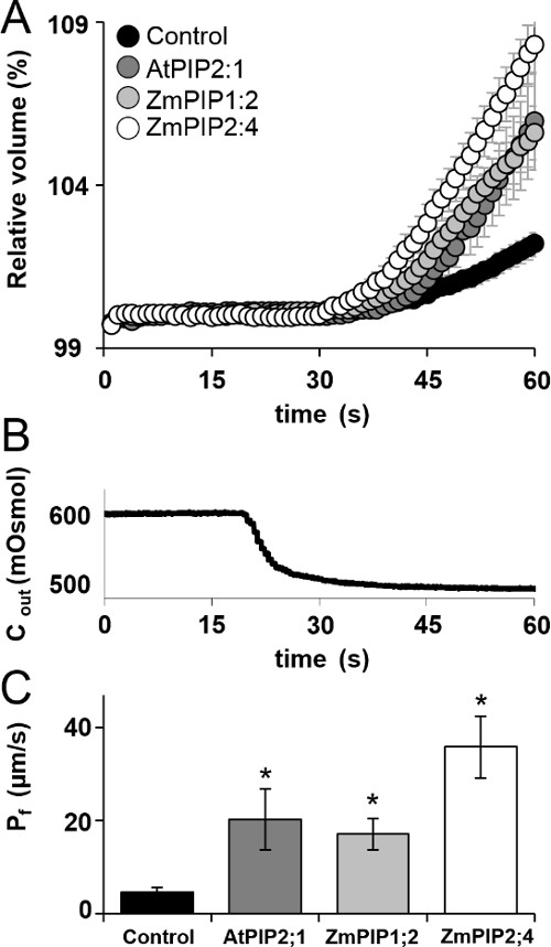
Figure 8: Volume change and the extracted osmotic water permeability, Pf. (A) Time course (60 sec) of protoplast swelling upon exposure to hypotonic challenge (mean ± SE). (B) The calculated osmoticum concentration in the bath during the hypotonic challenge. Note that while the hypotonic solution flow was switched on at 15 sec, it reached the bath only after a lag, here of 5.9 sec. (C) Pf (mean ± SE). Asterisks indicate significant differences from control (p ≤0.05). Data from at least three independent experiments for each treatment with a total of n protoplasts (control: n = 52, AtPIP2;1: n = 13, ZmPIP1;2: n = 28, ZmPIP2;4: n = 34).
