JoVE Science Education
Materials Engineering
Un abonnement à JoVE est nécessaire pour voir ce contenu.  Connectez-vous ou commencez votre essai gratuit.
JoVE Science Education Materials Engineering
Optical Materialography Part 2: Image Analysis
  • 00:08Vue d'ensemble
  • 01:01Principles of Image Analysis for Quantitative Materialography
  • 03:07Sample Preparation: Review
  • 03:47Pore Volume Measurement
  • 05:28Grain Size Measurement
  • 06:26Applications
  • 07:18Summary

Matérialographie optique II : Analyse d'image

English

Diviser

Vue d'ensemble

Source : Faisal Alamgir, School of Materials Science and Engineering, Georgia Institute of Technology, Atlanta, GA

L’imagerie des structures microscopiques des matériaux solides, et l’analyse des composants structurels représentés, est connu sous le nom de matériographie. Souvent, nous aimerions quantifier la microstructure interne tridimensionnelle d’un matériau en utilisant uniquement les caractéristiques structurelles démontrées par une surface bidimensionnelle exposée. Bien que les méthodes tomographiques basées sur les rayons X puissent révéler la microstructure enfouie (par exemple les tomodensitoyaux que nous connaissons dans un contexte médical), l’accès à ces techniques est assez limité en raison du coût de l’instrumentation associée. La matériographie au microscope optique offre une alternative beaucoup plus accessible et routinière à la tomographie aux rayons X.

Dans la partie 1 de la série Matérialogique, nous avons couvert les principes de base derrière la préparation de l’échantillon. Dans la partie 2, nous passerons en compte les principes qui sous-tendent l’analyse de l’image, y compris les méthodes statistiques qui nous permettent de mesurer quantitativement les caractéristiques microstructurales et de traduire l’information d’une section transversale bidimensionnelle à la structure d’un échantillon de matériel.

Principles

Procédure

Complétez toutes les procédures de Materialography Partie 1. Il convient de rappeler que la reproductibilité de ce qui suit ne peut être évaluée qu’en analysant plusieurs images d’un même échantillon. Si un logiciel d’analyse numérique est disponible, où les pixels peuvent être classés en fonction de leur luminosité et comptés en conséquence, alors il est possible d’utiliser l’équation [1] pour estimer le volume des pores en fonction de l’alt;A.. Sinon, cette analyse peut, bien sûr, se fair…

Résultats

In Figure 1 we see a cross section of a porous material with a grid superimposed on it. The points of intersection can be used to determine <Pp>. The number of intersection points that lie over dark regions (pores) is divided by the total number of intersection points to get Pp and by collecting and, by averaging Pp values from multiple images, we arrive at <Pp>.

Figure 1
Figure 1: Materialographic image with a superimposed grid. The intersection points on the grid are used for analysis.

Figure 2
Figure 2: Grains size measurements using lines at a) 0, b) 30, c) 60 and d) 90 degrees orientation. The grains are obviously anisotropic in shape (longer in one direction than the other). This anisotropy results from the nonuniform forces acting on the samples during processing through which the grains become "squashed".

Image ID Test points in porosity area Total no. of test points PP <PP>
Avg. Δ*
P1 32 100 0.32 29 1.77
P2 29 100 0.29
P3 22 100 0.22
P4 37 100 0.37
P5 24 100 0.24
P6 30 100 0.30

Table 1. Porosity measurements.

ID Probe L(mm) Horizontal (Radial or Hoop) Vertical (Axial)
I IL <IL> G I IL <IL> G
Avg. Δ
Avg. Δ*
SL1 0.9 16 17.7 18.1 0.68 0.05mm 3 3.33 3.7 0.31 0.27 mm
SL2 0.9 14 15.5 2 2.22
SL3 0.9 18 20 4 4.44
SL4 0.9 16 17.7 3 3.33
SL5 0.9 15 16.7 5 5.56
SL6 0.9 19 21.1 3 3.33

Table 2. Intercept measurements using straight line probes.

*: Δ is the sampling error. Assuming a confidence level of 95%, the sampling error can be estimated with the equation below:

Equation 7

N: number of samples

xi: the i th sample

µ: sample average

The probability of population average lying in the range [µ- Δ, µ+ Δ] is 95%. The sampling error can be used as criteria in telling if the difference between two averages is significant (e.g. the difference between the average of IL estimated with vertical line probes and horizontal line probes).

Applications and Summary

These are standard methods for analyzing two-dimensional cross sections in materials in order to extract three-dimensional information. We looked specifically at estimating the volume fraction of pores in one material and the average grain size in a second material.

Materialographic sample preparation described here are the necessary first step towards the analysis of internal microstructure of three-dimensional materials using two dimensional information. For example, one might be interested in knowing how porous a membrane material is since that will affect its gas pearmeability. An analysis of the void structure of the 2D cross section will provide a strong indication of what the porosity is in the actual 3D structure (provided the sampling statistics are high). Another application would be in analyzing, for example the orientation of the polycrystalline grains in oil pipeline alloys. The orientational distribution function (ODF) can be directly related to the axial and transverse mechanical strength of the pipes, and so our sample preparation procedure is an important component of such an analysis.

Transcription

Materialography is a method for microscopic structure imaging and analysis of structural components of solid materials. Quantitative image analysis methods, such as X-ray tomography, are helpful to characterize varied microstructures.

However, these often involve costly instrumentation. Optical microscope-based materialography is an affordable alternative to study solid materials. In a previous video on materialography, we covered the topic of sample preparation for optical materialography.

This video will now illustrate how to analyze the images of the prepared sample, using the principles of statistical methods and quantification of three-dimensional structure of a solid material.

From optical materialography, images are analyzed according to three main characteristics: porosity, grain density, and effective density.

Let us first look at the porosity. It is defined as the fraction of the volume of a material that is unoccupied by atoms. This void portion in a material determines its mechanical, electrical, and optical properties. It also affects its permeability. Statistically, the porosity is estimated on a representative two-dimensional slice of a sample, by the void area normalized by the total imaged area. By analyzing multiple images of the same sample, one obtains the mean void area of a sample. Similarly, by rasterizing the images, the average number of points, or pixels, line in void, normalized by the total probe points, gives the mean void points of a sample.

The second characteristic of polycrystalline materials is the grain density. Taking a rasterized image, it is estimated by quantifying the number of intersections of a grain with test lines. The mean number of intersections for all images is indicative of the average lateral dimension of a crystal grain. For high-porosity materials, the mean grain density can also be found through the mean porosity.

The third characteristic is the effective density. This takes into account the volume of pores in a material, and the global density of the material. Here the porosity can either be defined by the parameters A or P. We will now see how to analyze these three characteristics on images obtained from optical materialography.

The quantitative analysis of optical materialography images requires the pre-requisite procedure of sample preparation. Please refer to the video materialography part one for appropriate sample preparation protocol in four steps: cutting, mounting, polishing, and etching.

Let us now consider the prepared sample of a toroidal inductor core sample. Multiple images of the same sample are needed to perform the optical materialography analysis.

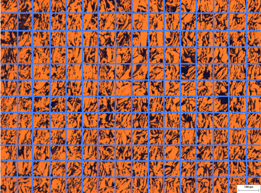
Use a digital analytical software where pixels can be categorized based on their brightness and counted accordingly. If not available, the analysis can be done by hand. Identify the void areas. Under Analyze in the menu, select Set Scale and choose the distance in pixels. Then select Image, Type, and 8-bit to change the image to grayscale. In the Process menu, select Binary and Make Binary to maximize the contrast of your image. Finally, choose Analyze Particles from the Analyze menu to measure the void area in micrometer units.

Take the sum of the void areas and normalize it by the total imaged area to obtain the parameter A. Repeat for all images to get the mean parameter A. Then, overlay a grid on the image. The intersection points are the test points. Count the number of test points. Identify porosity areas and count the total number of test points inside them. Normalize by the total number of test points to obtain the parameter P.

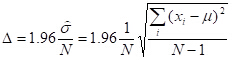
Repeat the calculation for all images to estimate the mean parameter P and the sampling error delta, where sigma is the standard deviation, n is the number of images, X-I is the sample I, and U is the sample average.

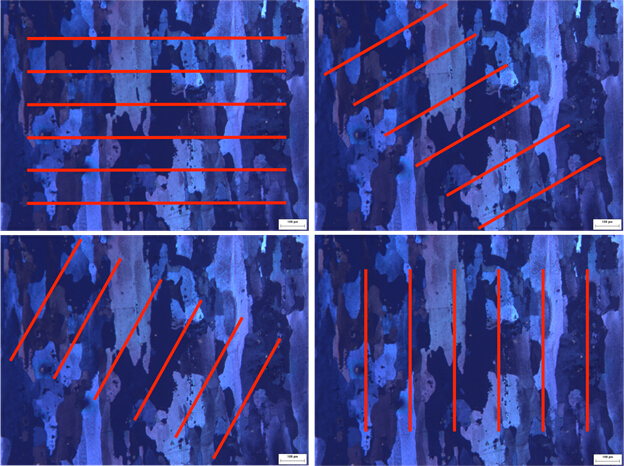
In the second step of the analysis, identify boundaries between neighboring grains, then superimpose a set of horizontal test lines on the image. Count the number of intersections between the test lines and the grain boundaries and evaluate the parameter I-L.

Repeat this step by rotating the lines by 90 degrees. Then repeat for all images. Calculate the mean intercept grain size in the horizontal direction and vertical direction. At last the grain size can be estimated.

Finally, rotate the lines at 30 degrees and 60 degrees and compare with previous vertical and horizontal cases. Observe the grain shape and the preferred angle of orientation. This is an indication of the anisotropy level of the sample.

Quantitative analysis of microscopic structure of solid materials with optical microscopy is useful for various applications. The study of grain size and shape in minerals contributes to the understanding of rock formation in extreme conditions.

For this reason materialographic analysis proves to be a useful method for planetary exploration. Polycrystalline samples may show various orientations of their grains. For example, in alloys used for oil pipelines, the orientational distribution function directly influences the axial and transverse mechanical strength of these alloys.

Materialography is routinely used to verify the quality of alloys that serve to build oil pipelines.

You’ve just watched Jove’s introduction to optical materialography. You should now understand the principles of image analysis used to investigate the microscopic structures of solids. You should also know how to determine porosity, grain size, and density for different materials.

Thanks for watching.

Tags

Cite This
JoVE Science Education Database. JoVE Science Education. Optical Materialography Part 2: Image Analysis. JoVE, Cambridge, MA, (2023).