Calorimétrie différentielle à balayage
English
Diviser
Vue d'ensemble
Source : Danielle N. Beatty et Taylor D. Sparks, Department of Materials Science and Engineering, The University of Utah, Salt Lake City, UT
La calorimétrie différentielle de balayage (DSC) est une mesure importante pour caractériser des propriétés thermiques des matériaux. DSC est utilisé principalement pour calculer la quantité de chaleur stockée dans un matériau pendant qu’il chauffe (capacité de chaleur) ainsi que la chaleur absorbée ou libérée lors de réactions chimiques ou de changements de phase. Cependant, la mesure de cette chaleur peut également conduire au calcul d’autres propriétés importantes telles que la température de transition vitreuse, la cristallinité des polymères, et plus encore.
En raison de la nature longue et en chaîne des polymères, il n’est pas rare que des brins de polymère soient enchevêtrés et désordonnés. En conséquence, la plupart des polymères ne sont que partiellement cristallins, le reste du polymère étant amorphe. Dans cette expérience, nous utiliserons DSC pour déterminer la cristallinité des polymères.
Principles
Procédure
Résultats
Figure 3 shows the result of a DSC percent crystallinity sample scan on a polybutylene terephthalate (PBT) polymer sample. The result is displayed as a DSC power reading (in milliwatts per milligram of sample) verses time. The power reading, the blue trace in Figure 3, indicates how much additional power was required to change the temperature of the sample pan in comparison to the empty reference pan. The temperature program is also displayed as the dashed red line in Figure 3. The first peak in the blue trace is an endothermic peak; its area gives a value for the heat of melting of the polymer sample. The second peak is an exothermic peak whose area gives a value for the heat of crystallization of the polymer sample.
Figure 4 shows zoomed views of the endothermic and exothermic peaks from the PBT scan (Figure 3). The area of each peak is shown (calculated using the Proteus Analysis software). From these calculated values, the percent crystallinity of this PBT polymer sample is calculated using Equation 1 and a reported value of 142 J/g for ΔHm°:
% Crystallinity = 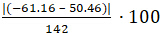 = 78.6% crystalline
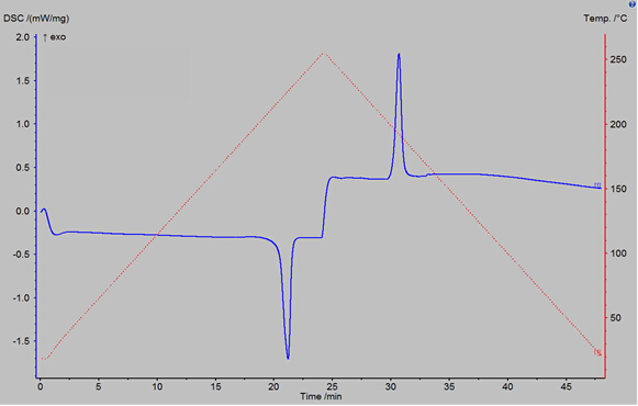
Figure 3: DSC reading vs time for a polybutylene terephthalate polymer sample, run using the DSC 3500. The temperature program used is also shown as the red dashed curve.
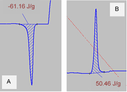
Figure 4: Zoomed view of the endothermic peak (A) and the exothermic peak (B) of PBT polymer DSC scan. Areas under each curve are calculated; these correspond to the heat of melting and heat of cold crystallization of the PBT polymer sample, respectively.
Applications and Summary
Differential scanning calorimetry is a technique used to determine many thermal properties of materials, such as heat of melting, heat of crystallization, heat capacity, and phase changes. DSC measurements can also be used to calculate additional material properties including glassy transition temperature and polymer percent crystallinity. The DSC requires very small samples that must conform to the size and shape of the pans used in the machine and is based on a differential heat comparison between an empty reference and a sample. Polymer percent crystallinity calculations are relatively simple if the heat of melting of a 100% crystalline form of the polymer being tested is known. Other characterization methods that can determine percent crystallinity include density measurements, which also require a 100% crystalline and a 100% amorphous version of the polymer, and X-ray diffraction, which requires a sample that can be thoroughly mixed with a standard material such as silicon.
Percent crystallinity is an important parameter that significantly contributes to many of the properties of polymer materials used every day. Percent crystallinity plays a role in how brittle (high crystallinity) or how soft and ductile (low crystallinity) a polymer is. Polyethylene is one of the most widely used polymer materials and is a good example of the importance of crystallinity to material properties. HDPE (high density polyethylene) is a more crystalline form and thus is a harder, more brittle plastic used in garbage bins and cutting boards, whereas LDPE (low density polyethylene) has a lower crystallinity and is thus a ductile plastic used in disposable plastic shopping bags. Polymer crystallinity can also affect transparency and color; polymers with higher crystallinity are more difficult to color and are often more opaque. Percent crystallinity plays a large role in how we create and use different plastics and different forms of the same plastic every day, from polymers used in fabrics, to those used in bullet proof vests. Other polymeric characteristics that can affect these properties, and can contribute to percent crystallinity values, include previous heat treatments and degree of crosslinking.
Transcription
Differential scanning calorimetry or DSC is an important measurement technique used to characterize the thermal properties of materials especially polymers. The DSC measurement set-up consists of separate sample and reference pans, each with identical temperature sensors. The temperature of the sample pan containing the sample of interest and the reference pan which typically remains empty are controlled independently using separate but identical heaters. The temperature of both pans is increased linearly. The difference in the amount of energy or heat flow required to maintain both pans at the same temperature is recorded as a function of temperature. For example, if the sample pan contains a material that absorbs energy when it undergoes a phase change or reaction the heater under the sample pan must work harder to increase the pan temperature than the heater under the empty reference pan. This video will demonstrate how to use DSC to determine polymer phase transitions and calculate the percent crystallinity of a polymer.
Due to the long chain-like structure of polymers the strands can exhibit long-range order and are called crystalline or can be randomly organized, termed amorphous. Crystalline polymers undergo a phase transition from solid to liquid through melting. Whereas amorphous polymers transition from their rigid state, called a glass, to their rubbery state through a glass transition. These events can be measured using DSC. However most crystalline polymers are only partially crystalline with the remainder of chains being amorphous. These are called semi-crystalline polymers. In these materials the amorphous parts of the polymer undergo a glass transition during heating while the crystalline parts undergo melting.
These events are visualized in a DSC curve of heat flow versus temperature. Exothermic changes, meaning those that give off heat, are shown as peaks in the plot. While endothermic events, those that absorb heat, appear as valleys. Those peaks and valleys are specific to the certain phase changes in a polymer. The heat of melting, delta Hm, is the amount of energy required to induce melting in a crystalline polymer when the temperature increases. We can calculate the heat of melting by taking the area under the endothermic peak during the heating phase of the measurement.
The heat of cold crystallization, delta Hc, is the amount of energy released as the sample cools and re-crystallizes. Delta Hc is calculated using the area under the exothermic peak during the cooling phase of the measurement. So if we heat the sample past melting and then cool back to room temperature, we can determine both delta Hm and delta Hc. Then using this relationship, we can determine the percent crystallinity. Now that you’ve seen how to identify phase changes in a DSC plot, let’s take a look at how to run the measurement and analyze the results.
To begin the DSC measurement switch the instrument on and allow it to warm up for about an hour. Check that the compressed nitrogen tank and liquid nitrogen tank are both full and that the valve connecting them are open. Now prepare the two pans. Choose a pan that is chemically inert and stable in the desired temperature range. Poke a small hole in the lids. Place the lids on each pan, and then seal them using a crimping press. Next remove the three furnace covers and place the two empty pans on the circular sensors within the furnace. Then replace the furnace covers. Launch the DSC software on the computer and create a new file.
The Measurement Definition window will open with tabs to define measurement parameters. Select Header and then Correction under Measurement Type. This will save the baseline measurement as a correction file which will be subtracted from the sample measurement by the software. Under the Sample section label the baseline measurement and date. Then under temperature calibration, select the most recent temperature calibration file. For a percent crystallinity measurement under Sensitivity Calibration, select the most recent sensitivity calibration file. Then under the temperature program tab, check the Purge2 and Protective boxes under the Step Conditions. This turns the nitrogen purge gas on for all temperature steps.
Select Initial under the Step Category and input 20 degrees Celsius as the start temperature. Then select Dynamic and input in an end temperature. It should be about 30 degrees higher than the reported melting temperature of the polymer sample. In this case we will use 260 degrees Celsius. Then click on the drop-down arrow under the liquid nitrogen icon to set up the cooling step. Select auto to automatically turn on the liquid nitrogen to cool the furnace after the heating step has finished. Select Final under the Step Category and input 20 degrees as the end temperature. Then set the Emergency Reset Temperature 10 degrees higher than the highest temperature in your program which shuts off the instrument in case of machine malfunction and overheating. Now with all of the parameters set, check the initial temperature that you defined and the current furnace temperature. To start the program, the furnace must be within five degrees of the initial temperature. Click Start to begin heating and the program will begin automatically.
After the baseline scan has run remove the empty baseline pan from the furnace. Obtain a new pan and lid and poke a hole in the lid. Weigh the empty sample pan and lid. Then cut the polymer sample into small pieces that will fit in the pan. To ensure even heat flow place a thin layer of the sample pieces in the pan so that the entire bottom of the pan is covered. Then place the lid on the pan and crimp it closed. Now weigh the full sample pan and subtract the weight of the empty pan to determine the weight of the sample.
Then place the pan in the furnace and close the cover. In the DSC software, select File, then Open. Click OK when the program asks to open the baseline scan. On the measurement definition window select Correction + sample under the Measurement Type. Then under the sample section input the sample name and mass. Select Forward and press Start when prompted to begin the scan. After the measurement has finished close the program, turn off the compressed nitrogen tank, and then turn off the instrument.
The DSC data of the polymer sample polybutylene terephthalate is presented as a plot of heat flow versus time. The red trace shows the increase of temperature to 260 degrees, and then the cooling back down to room temperature. Here the curve shows two distinct peaks. The first peak occurred during heating and is an endothermic peak corresponding to the heat of melting. The heat of melting is calculated using the area under the curve which equates to about minus 61 joules per gram. The second peak is an exothermic peak which occurred during the cooling step and corresponds to the heat of cold crystallization. The heat of crystallization is calculated by taking the area under the curve which is about 50 joules per gram. With these two values, along with the known heat of melting for a 100% crystalline sample of polybutylene terephthalate, we can calculate the percent crystallinity of the sample which is 78.6%.
DSC can be used to study thermodynamic events in other samples and materials as well. For example, DSC can be used to analyze phase transitions in biological samples. In this experiment the phase transition of a cell suspension was analyzed in order to understand its freeze-drying properties. Freeze-drying or lyophilization is commonly used for long-term storage of biologicals. Here cell suspensions were prepared and frozen under different conditions in the DSC instrument. The frozen suspensions were then heated and the glass transition measured. Later, the cells were analyzed with electron microscopy to determine which freezing condition promoted cell survival. An understanding of the freeze-drying process via phase transition temperatures helps tailor the process in order to improve cell storage.
The enthalpy change occurring during a chemical reaction is a measure of the amount of heat absorbed in the case of an endothermic reaction or released in the case of an exothermic reaction. The enthalpy change during a reaction can be measured using DSC by performing the chemical reaction inside of the sample pan and measuring the heat flow. In this example, the enthalpy of decomposition of calcium carbonate to form calcium oxide or quicklime was measured by DSC. The decomposition of calcium carbonate occurs endothermically as evidenced by the positive peak at 853 degrees Celsius. The enthalpy of decomposition of calcium carbonate is calculated from the area under the peak and is approximately 160 kilojoules per mole.
You have just watched JoVE’s introduction to studying polymer phase transitions using differential scanning calorimetry. You should now understand the different phase transitions for a crystalline and amorphous polymer, and how to identify the events, and calculate crystallinity using DSC. Thanks for watching.