JoVE Science Education
Materials Engineering
Un abonnement à JoVE est nécessaire pour voir ce contenu.  Connectez-vous ou commencez votre essai gratuit.
JoVE Science Education Materials Engineering
Electrochemical Impedance Spectroscopy
  • 00:08Vue d'ensemble
  • 01:35Principles of Electric Impedance Spectroscopy
  • 04:21Measuring and Modeling Impedance
  • 06:20Calculating Impedance
  • 07:24Applications
  • 08:28Summary

Espectroscopia de Impedância Eletroquímica

English

Diviser

Vue d'ensemble

Fonte: Kara Ingraham, Jared McCutchen, e Taylor D. Sparks, Departamento de Ciência e Engenharia de Materiais, Universidade de Utah, Salt Lake City, UT

Resistência elétrica é a capacidade de um elemento de circuito elétrico resistir ao fluxo de eletricidade. A resistência é definida pela Lei de Ohm:

Equation 1(Equação 1)

Onde Equation 2 está a tensão e é a Equation 3 corrente. A lei de Ohm é útil para determinar a resistência dos resistores ideais. No entanto, muitos elementos de circuito são mais complexos e não podem ser descritos apenas pela resistência. Por exemplo, se uma corrente alternada (AC) for usada, então a resistividade dependerá muitas vezes da frequência do sinal CA. Em vez de usar apenas a resistência, a impedância elétrica é uma medida mais precisa e generalizada da capacidade de um elemento de circuito de resistir ao fluxo de eletricidade.

Mais comumente, o objetivo das medidas de impedância elétrica é a desconvolução da impedância elétrica total de uma amostra em contribuições de diferentes mecanismos, como resistência, capacitância ou indução.

Principles

Procédure

Obtenha um módulo de teste e conecte-o aos instrumentos EIS através de dois eletrodos. O módulo de teste, retratado na Figura 3,fornece dados que podem ser usados para modelar um circuito simples e conhecido. Pode ser usado para confirmar que os fios estão ligados à máquina corretamente e que todas as peças de máquinas estão funcionando. Figura 3: Módulo de te…

Résultats

Results of EIS are often presented in a Nyquist plot, which shows real impedance versus complex impedance at each frequency tested. The plot of the experiment ran can be seen in Figure 6.

Figure 6
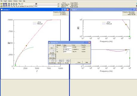
Figure 6: Screenshot of computer after Nyquist plot was obtained. 

As seen in step 9 of the procedure, the software will give you options of circuits to model your data. It is best to choose the simplest model that still accurately reflects the data. Choosing the correct circuit to model the data is a difficult, inverse problem. While software packages exist that can assist in generating model circuits, care should be taken during this analysis.

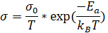
When an equivalent circuit is chosen, the resulting data can be used to calculate the conductivity of the sample. One way to calculate conductivity is to plot the data from EIS using an Arrhenius model, which plots 1000/T on the x-axis and log(σT) on the y-axis. The data can be fitted to a linear line using the following equation:

Equation 13    (Equation 5)

Where Equation 14 for our sample was 374 S/cm*K and Ea, the activation energy, was 0.17 eV, and T = 298 K. Plugging in these values, we calculated a conductivity of 1.67 x 10⁻³ S/cm. Previous experiments with this sample reported its conductivity to be approximately 4.1 x 10⁻³ S/cm. This is fairly similar to the conductivity value we calculated, indicating that the model we chose was a good, though not perfect, fit.

Applications and Summary

Electrochemical Impedance Spectroscopy is a useful tool for determining how a new material or device impedes the flow of electricity. It does this by applying an AC signal through the electrodes connected to the sample. The data is collected and plotted by the computer in the complex plain. With the help of software, the graph can be modeled after specific parts of a circuit. This data can often be very complicated and requires careful analysis. This technique, however complex, is an extremely useful non-destructive means of interrogating the real world complexities of electrical impedance, and can provide useful models of how AC current behaves when applied to the sample.

EIS can be used to look at microorganisms in a sample. When bacteria grow on a sample, it can change the electrical conductivity of the sample. Using this idea, you can measure the impedance of a sample at one frequency to determine the population of microorganisms. This technique is known as impedance microbiology.

EIS can also be used to screen for cancer in tissues, known as Tissue Electrical Impedance. The electrical impedance of bodily tissue is determined by its structure. As it degrades over time, it's impedance of electrical current also changes. Much like impedance microbiology, this type of impedance testing looks at the population of cells and can provide useful information about cell heath and morphology.

EIS is also used in the paint and corrosion prevention industries to determine how well a layer is applied to the surface of a material. EIS data corresponds well to every day electrochemical processes that attack surfaces; materials that show an electrical resistance of less than Equation 15 may not protect against corrosion as well as materials with a higher resistance. EIS is an avenue to predict how new surface treatments will fair in harsh environments without having to recreate them, making it an invaluable tool in the prevention of corrosion which would otherwise cost the United States billions of dollars in repairs every year.

Transcription

Electrochemical impedance spectroscopy is a powerful technique used to characterize materials based on how they impede the flow of electricity in applications as diverse as microbiology and corrosion resistance. The electrical conductivity of a sample is based on the make up of all of the components of the sample. Because of this, EIS can also be used to detect changes in the quantity or structure of each component. EIS is performed by applying a small sinusoidal electrical load across electrodes connected to a sample at a wide range of frequencies. Based on the measured response, impedance is computed at each of the frequencies. Computer software is then used to plot the results and build an equivalent circuit model that is representative of the observed data. The typical goal of using EIS is breaking down the sample’s total electrical impedance into contributions from mechanisms such as resistance, capacitance, or induction. This video will illustrate the principles and procedures involved in EIS to determine the impedance of a material. It will also demonstrate how to create equivalent circuit models of the sample.

Electrical resistance is the ability of a circuit element to resist the flow of electricity. And Ohm’s Law defines resistance as voltage divided by current. When dealing with AC currents, however, electrical impedance is a more accurate and general measure of the ability to resist the flow of electricity. This is because, in addition to the resistance of the material, it accounts for the contribution of mechanisms, such as capacitance and induction. If an applied AC signal is sinusoidal and the response is linear, the current produced will also be sinusoidal, but shifted in phase. To account for the frequency and phase shift we can build impedance equations for components of a circuit using Euler’s Relationship and complex numbers. These models are used to interpret data showing impedance to be independent of frequency for resistors, inversely related to frequency for capacitors, and directly related to frequency for inductors. During EIS testing, the instrument applies an alternating field voltage to a sample and measures the current response. The real and imaginary components of impedance are calculated by determining the phase shift and change in amplitude at different frequencies. A Nyquist plot is generated by plotting the imaginary component on the Y axis and the real component on the X axis. One of the simplest Nyquist plots is a semi circle. The plot is then used to build a circuit model that best represents the impedance of the sample. During modeling, physical processes correspond to elements of a circuit. For example, an electrical double layer corresponds to a capacitor. The equivalent circuit model for this plot is represented by a resistor in series with a resistor and capacitor in parallel. This is a common starting place for the interpretation of a Nyquist plot. The software will present you with equivalent circuit models based on your Nyquist plot for you to choose from. If these models do not fit your data you can manually model a circuit to fit the data, a complicated task. In the next section, we will show you how to test a control sample and an experimental sample with EIS and then build an equivalent circuit to represent the observed impedance data.

Gather EIS instruments and a test module. Hook the test module up to the EIS instruments via two electrodes to model a simple known circuit. Open the ZPlot software on the computer to set the parameters for the test module. Set DC potential to zero, AC amplitude to 10 millivolts, and the drop down arrow to versus open circuit. Set initial frequency to one times 10 to power six hertz, final frequency to 100 hertz, and interval to 10. Select logarithmic and steps per decade. Measure, then sweep, to start a new recording, and begin collecting data. Compare measured values to expected values found on the front of the test module. If the values do not match, check wiring and equipment, and retest. Obtain the sample of beta alumina and put it in the assembly. Working in the fume hood, insert the assembly into the tube furnace and attach the electrodes. Open the ZPlot software keeping the same parameters used for the test module and press measure, then sweep. Open the ZView software to view the results as you did for the test module. Save the plots. Choose two points to fit the semi circle. Then press the instant fit button to choose the best equivalent circuit model. For simplification, we ran this experiment at room temperature. EIS tests are usually run by varying amplitude or voltage as well as temperature.

Let’s now take a look at our results. Results of the EIS are presented in a Nyquist plot showing real impedance versus complex impedance at each frequency tested. Multiple options of circuits to model your data are provided, it is best to choose the simplest model that still accurately reflects the data. Next, choose an equivalent circuit, and using the resulting data, let’s calculate the conductivity of the sample. Data can also be fitted to a linear line using the equation for conductivity. Using the values found through repeated testing for this sample, a conductivity of 1.67 millisiemens per centimeter is calculated, as compared to the reported conductivity value of approximately 4.1 millisiemens per centimeter. This indicates that the model we chose was a good, though not perfect fit.

Now that you appreciate the methods of measuring and modeling impedance using electrochemical impedance spectroscopy, let’s take a look at some of the applications for this tool. EIS can be used to look at microorganisms in a sample. When bacteria grow on a sample it can change the electrical conductivity of the sample. Because of this, EIS can be used to measure impedance to determine population growth. This technique is known as impedance microbiology. EIS is also used in the paint and corrosion prevention industries. Materials that show an electrical resistance of less than 10 to the power six Ohms per centimeter square may not protect against the electrical chemical processes that attack surfaces everyday. EIS testing predicts the corrosion resistance properties of materials to be used in harsh environments, saving billions of dollars in repairs every year in the United States alone.

You’ve just watched JoVE’s introduction to electrochemical impedance spectroscopy. You should now understand how to test and model the impedance characteristics of materials. Thanks for watching.

Tags

Cite This
JoVE Science Education Database. JoVE Science Education. Electrochemical Impedance Spectroscopy. JoVE, Cambridge, MA, (2023).