Science Education
>

Live Cell Imaging of Alphaherpes Virus Anterograde Transport and Spread

PRÉPARATION DE L'INSTRUCTEUR
concepts
PROTOCOLE ETUDIANT
Journal JoVE
Immunologie et infection
Un abonnement à JoVE est nécessaire pour voir ce contenu.  Connectez-vous ou commencez votre essai gratuit.
Journal JoVE Immunologie et infection
Live Cell Imaging of Alphaherpes Virus Anterograde Transport and Spread

Section 1 – Environmental Control Conditions for Live-cell Fluorescence Microscopy

  1. 30 min prior to any imaging experiment connect and begin warming the microscope stage top incubator.
    1. Turn on microscope, transmitted and epifluorescent light sources, and automated hardware controls. Open the microscope control software, NIS Elements, to connect to the microscope and begin cooling the EM-CCD camera.
    2. Attach Lens warmer to appropriate objective (either 60X or 100X oil immersion). Note: Select objective lens based on experiment type. The 100X differential interference contrast (DIC) is best for tracking of anterograde transporting virion assemblies while the 60X phase objective is suited to visualize anterograde spread. Lower magnification, non-oil immersion objectives do not require a lens warmer as they do not make direct contact with the sample.
    3. Attach stage top incubator onto the motorized stage of microscope. Ensure the appropriate insert that will hold the sample is in place. Attach the humidified air line from the incubator control to the input port on the stage top incubator.
    4. Turn on incubator and lens warmer controls and adjust temperature settings to previously verified conditions specific for the objective and sample being imaged (see discussion).
    5. Open the control valve on the 5% CO2/95% atmospheric tank to provide CO2 supplemented air to stage top incubator. The flow rate should be between 60 and 80 ml of gas per minute. Faster rates will result in extensive sample dehydration despite the humidifying chamber.
  2. Add lens oil to objective lens and immediately place the culture that will be imaged into the stage top incubator.
  3. Allow equilibration of temperature in the culture for a minimum of 10 min. One hour is preferred, especially for overnight imaging described in Section 3.

Section 2 – Real-time Imaging of Anterograde Virion Transport Events Protocol

  1. Six to eight hours prior to imaging, infect a 35 mm coverslip-bottom dish of mature, dissociated SCG neurons with 1 x 10⁶ plaque forming units of the virus of interest (See Table 1 for example viruses) using the method described in Taylor et al. 2012a 11. If testing more than one virus, off-set inoculations by 30-60 min to allow for imaging of sequential samples at similar times post infection.
  2. Insert dish into stage top incubator for a minimum of 10 min before running any experiment. While the temperature equilibrates, the focal plane is shifting and will negatively impact any imaging experiments.
  3. Using transmitted light and the eyepiece of the microscope, find a neuronal cell body that has a clearly isolated axonal extension. Alternatively, use the appropriate fluorescence illumination to find a cell expressing detectable amounts of fluorescent proteins. It is important to limit exposure of sample to fluorescent illumination, at this step and subsequent steps, because of light induced cellular damage and bleaching of fluorescent proteins.
  4. Attenuate fluorescence illumination to reduce the intensity of excitation light to which the cells are exposed. Engage light attenuating Neutral Density (ND) filters in the fluorescence illumination light path. For movies lasting longer than 1 min, a minimum of ND4 must be used to prevent photo-bleaching of fluorescent proteins and extensive photo-damage of axons. Highly fluorescent structures can typically be visualized with an ND8 filter in place.
  5. Using the microscope software (Figure 2 and Supplemental Movie 1A), switch the light-path to the EM-CCD camera.
  6. Determine optimum imaging times and conditions for each fluorescent channel.
    1. Initiate a live image window using the “Play” button.
    2. Determine the optimal camera exposure settings for each fluorescent protein. Do not exceed 300 msec per channel as motional aberrations of fast moving virion structures will occur. Utilize the EM gain of the camera to a setting of 300 (manufacturer suggested maximum gain), to minimize exposure time and enhance detection of dim signals. Correct exposure times should produce an image with low background intensity and high specific signals.
  7. After setting exposures and finding a well-defined region of axon, the software must be configured to perform automated image acquisition. Stop the live imaging window to prevent sample bleaching.
    1. In the NIS Elements software, select the 6D – Define/Run Experiment application from the “Applications drop down menu.
    2. In the ND acquisition window, click the Time tab which will determine the frequency of image acquisition. Set the Interval to “No Delay” and the Duration to 5 min. The software will then acquire image frames at the highest frequency possible for duration of 5 min.
    3. Select the “Lambda” tab, which allows selection of the pre-set hardware configurations used for multiple fluorescent image acquisition. Click the first box and in the subsequent drop down menu to select an appropriate hardware configuration. Repeat for all fluorescent proteins to be imaged.
    4. Ensure the tabs for “XY Positions”, “Z-series” and “Large Image” are de-selected.
    5. Above the tabs, select the box marked “Save to File” to automatically save images to the hard disk during acquisition. Configure the location and file name of the experiment output file. As sequential experiments are performed, the software will add a sequential number at the end of the designated file name.
    6. Once all tabs have been selected. Initiate the experiment by clicking the “Run-Now” button.
    7. Optimize the image acquisition rate through exposure settings and image size. Using a small region of the image-able area will often speed up frame acquisition rates. Define the Region of Interest using the ROI tool in NIS-Elements, selecting an area between 25% and 50% of the total image area. Alternatively, shorter exposure times will increase frame acquisition rates, but decreases the quality of signal (see discussion).

Section 3 – Overnight Time-lapse Imaging of Anterograde Spread Events

  1. Four hours prior to imaging, infect a compartmentalized neuronal culture constructed on a 35 mm μ-Dish. Inoculate neuronal cell bodies with 1 x 10⁶ plaque forming units of the virus of interest (See Table 1 for example viruses) using the method described in Taylor et al. 2012b 12.
  2. Gently place culture dish into the stage top incubator. Ensure the position of the objective is set to the side of the dish. Slowly bring the objective into focus, ensuring the objective does not push up into the sample. Once the focus field has been identified, slowly move the objective into the center of the dish, near the internal barrier demarking the internal side of the axon compartment. During movement, ensure the focus depth is maintained and avoid pushing up into the sample. Deflection of the plastic surface by the objective will damage the axons and the plastic.
  3. Add approximately 2 ml of warm (~37 ° C) phosphate buffered saline to the culture dish outside of the Teflon ring. This surrounds the neuronal culture with a ring of PBS to minimize sample dehydration and provide thermal insulation.
  4. Allow temperature to equilibrate for a minimum of 1 hr prior to initiating automated image acquisition (3.8). Steps 3.5 through 3.7 can be configured during this time.
  5. Restrict the intensity of illumination to the lowest possible level by engaging all neutral density filters. This will allow frequent image acquisition over long time periods without excessive photo-damage. Reducing illumination will result in low signal, requiring longer exposures (see discussion).
  6. Use historical exposure settings or prior to experimental set-up generate a parallel dish of infected epithelial cells expressing the target fluorescent proteins to establish exposure settings as described in Section 2.5.
  7. After setting exposures for the necessary channels, it is time to configure the software for automated image acquisition. Stop the live imaging window to limit sample bleaching.
    1. In Elements software (Figure 2 and supplemental movie 2), select the 6D – Define/Run Experiment application from the “Applications drop down menu to bring up the ND Acquisition window.
    2. In ND Acquisition window, click the Time tab. Set the Interval to “5 min”. Set the Duration to 20 hr. The loops field will be automatically calculated for the number of repetitions the program will perform.
    3. Select the “Lambda” tab. Click the first box and in the subsequent drop down menu select the appropriate lambda configuration for Phase contrast. Repeat for subsequent positions, selecting the appropriate configurations for each fluorescent protein to be imaged.
    4. Select the “Large Image” tab, which determines the parameters of multiple images to be combined into a single larger field of view. A good-sized area consists of 5 x 2 images using a 7% stitching overlap. This will allow for the maximum number of cells per position to be imaged without impacting the frequency of image acquisition. Also, deselect the checkbox for “Close Active Shutter during Stage movement”. This option enhances the speed of acquisition by not closing shutters between images.
    5. Select the “XY Positions” tab, to identify multiple positions that will be sequentially imaged in parallel during the course of the overnight movie. Select positions that define the center point for each large image area. Select 6-8 image positions in the sample. A good image area will have small clusters of cells in close apposition to clearly defined axons. Cells should not be piled on top of each other and axon bundling should be minimized. The point of focus is the nucleus of the cell. Position the objective such that a clearly defined nuclear envelope is seen for the majority of the cells.
    6. Ensure the “Z-series” tab is deselected.
    7. Configure the auto-save feature as described above in Section 2.6.5.
    8. Test the exposure and position settings by clicking “1 time loop. Evaluate the resulting images for transmitted light illumination, focus, and framing. If focus has shifted, reset the focus for each position under the X-Y tab. Wait 10 min and repeat this step until focus is stable.
    9. After all settings have been verified and tested, initiate the automated experiment by clicking the “Run Now” button.

Section 4 – Image Processing and Export

Data Export

  1. Datasets obtained during live-cell imaging of transport or spread events should be exported from the NIS Elements software into commonly used file types for later use in presentations and publications (Supplemental Movie 3). To export movies open the appropriate raw .nd2 file in NIS Elements and select the “split-component” view to visualize the desired fluorescent channels. Playback the file at a suitable speed; 5 frames per second is a good starting point for visualization of fast-transport.
  2. Include a timestamp to represent a real-time clock during movie playback. Right-click on the image and select, Add ND-information. A digital counter will appear in the upper left corner.
    1. Edit the time-stamp to display information. Right click on the counter and select Edit ND-information. In the subsequent pop-up window, edit the text to reflect the imaging parameters that are important. Edit font, color and size for clarity.
  3. Go to the “Edit” menu and find “Create view snapshot” or press the “x” key. This command opens the “view snapshot” window. Select “apply to all frames” to generate an 8-bit, RGB, export-ready file containing the fluorescent channels from the entire movie.
  4. Save as an .avi file for cross-platform compatibility. Set playback rate at 200 msec per frame. The .avi files generated by NIS Elements can then be further compressed with other conversion software into the desired file type.

Live Cell Imaging of Alphaherpes Virus Anterograde Transport and Spread

Learning Objectives

Anterograde Transport

Application of this protocol to infections of dissociated SCG cultures with PRV 348, a recombinant PRV strain expressing GFP-Us9 and gM-mCherry membrane fusion proteins, has facilitated the visualization of the anterograde transport of virions (Figure 3 and Supplemental Movie 4). Incorporation of these fusion proteins into viral particles results in their detection on transporting puncta, and the aforementioned imaging conditions minimize the offset of each fluorophore on a moving particle during filter switching. In a three-minute imaging window, numerous transporting puncta are commonly observed and large sample sizes for colocalization analyses are rapidly generated. We have previously quantified the colocalization of GFP-Us9, the alphaherpes virus axonal targeting protein, with other structural proteins using this approach 11. Similar analyses of other dual recombinant PRV strains have also been described 11, and recent work has documented the co-transport of PRV proteins with a fluorescently tagged host motor protein in a further extension of this protocol 21. Utilizing fast switching filter wheels and paired multi-pass dichroic mirrors allows rapid sequential acquisition of two or more fluorescent channels. We can currently achieve two-channel sequential acquisition at speeds of up to 0.8 frames per second. For single channel video microscopy, which is limited only by the fluorescence exposure time and read-time of the camera, we can achieve acquisition rates greater than 6 frames per second.

Anterograde Spread

To visualize anterograde spread events, areas of interest are visualized every 5 to 10 min for a 20 hr period, during which time virions will transport down and egress from axons, infecting the nearby epithelial cells. A representative frame from the large image area is presented in Figure 4A and Supplemental Movie 5. Note the spatially separated nature of the fluorescent protein expressing cells, indicative of primary infection from axons. Infected cells can be tracked backwards during the movie to visualize the fluorescent capsids that initiated the viral infection. These individual cells can be isolated from the large frame and tracked without a significant loss of detail. The representative frame (Figure 4B) from Supplemental Movie 6 depicts a time after virions have deposited the fluorescent capsid into the cytoplasm.

Data Analysis

A range of different analyses can be performed on live-cell imaging datasets including particle tracking, colocalization studies, and quantification of virion spread events. We often perform our analyses directly in the NIS Elements software or utilizing a plug-in extension available for the ImageJ software package that enables .nd2 file type support. Different hypotheses and experimental setups necessitate unique analytical methods. Our group has described methods for assessing colocalization of fluorescent proteins on dynamic structures 11,21 and time-lapse quantification of individual particle spread events 10,12,22. The methodologies describe in this manuscript and our previous studies are flexible and can be applied to different viral infections as well as the transport of cellular structures, e.g. mitochondria 23.

Figure 1
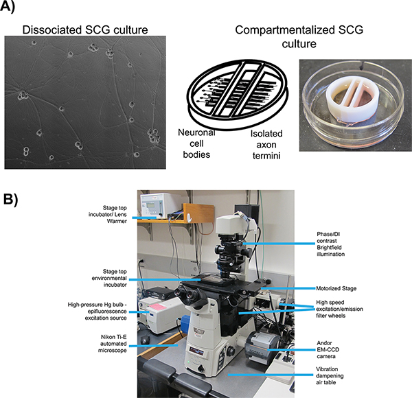
Figure 1. Schematic of microscopy set up for live cell imaging. A) Culture types employed for studies of anterograde transport (dissociated) and anterograde spread (chambered) respectively. Panel 1 is a phase contrast image of a mature, dissociated Superior Cervical Ganglia (SCG). Panel 2 is a schematic of the compartmentalized culture system, pictured in panel 3, with SCG neurons plated in the left compartment with axonal projections extending beneath the internal barriers into the far right compartment. B) The inverted epifluorescent microscope and stage top incubator configuration used for video microscopy experiments. Click here to view larger figure.

Figure 2
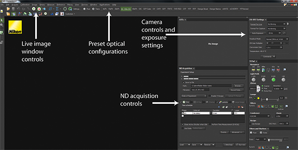
Figure 2. NIS-Elements software interface. A screenshot of a standard user interface in NIS-Elements is displayed. The Play and Stop buttons control the live-image window depicting the current hardware configurations for imaging as well as what is currently being imaged. Across the top panel are a series of Optical Configurations that implement preset hardware settings to configure the microscope for trans-illuminated or fluorescence detection. The Camera control and exposure settings allow configuration of camera detection to optimize image quality and speed. All experiments are coordinated using ND Acquisition controls. Click here to view larger figure.

Figure 3
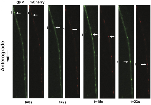
Figure 3. Live cell imaging of SCG axons at 8 hr post-infection with PRV 348. PRV 348 infected neurons express the GFP-Us9 and gM-mCherry membrane fusion proteins. Anterograde-transporting structures within distal axons are visualized in two fluorescent channels, GFP and mCherry. An anterograde-transporting structure (white arrow) progresses within the axon as depicted in the sequential images taken from Supplemental Movie 4. The two fluorescent proteins are spatially off-set due to sequential acquisition of fluorescent channels and the rapid movement of viral structures. Click here to view larger figure.

Figure 4
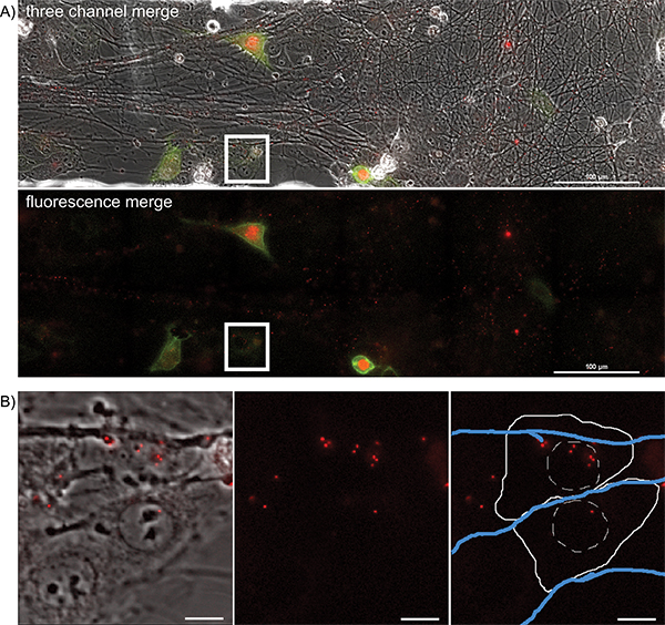
Figure 4. Overnight timelapse imaging of anterograde spread events from infected axons to epithelial cell clusters during a multi-color infection. Representative images from a single position, large image tiled time-lapse movie of virion transmission from PRV 427 infected axons into recipient epithelial cells. A) A merged image of the transmitted, YFP and RFP fluorescent images at a time post infection where recipient cells are beginning to express the YFP-CAAX and VP26-mRFP fusion proteins. In the second panel, the YFP and RFP channels are shown together. Note the large number of mRFP puncta associated with the axon tracts. These are assembled virions undergoing long distance transport within axons (Supplemental Movie 2). The white box represents the area of interest highlighted in part B. B) Representative image of recipient epithelial cells containing infecting capsid assemblies (See also Supplemental Movie 3). Panel 1 is a merge of the transmitted and RFP channels. Panel 2 is the RFP channel alone. Panel 3 is the RFP channel with a schematic representation of the cell outline (solid white line), nucleus (hashed white line), and axons (blue lines). Click here to view larger figure.

Supplemental Movie 1. Software settings for rapid, sequential acquisition of axonal virions. The steps associated with determining exposure settings, configuring ND acquisition controls, and acquiring a rapid frame acquisition movie of fluorescent virions undergoing axonal transport is presented. The SCG neuron culture was infected with PRV 427 eight hours prior to imaging. Click here to view movie.

Supplemental Movie 2. Software settings for overnight imaging of axon-to-cell spread. The steps associated with configuring ND acquisition controls for overnight imaging of axon-to-cell spread events are presented. Click here to view movie.

Supplemental Movie 3. Conversion of .nd2 files into presentable movie formats. The steps associated with converting the raw data .nd2 files into either .avi or .mov file formats for presentation using common video players. Click here to view movie.

Supplemental Movie 4. Live cell imaging of SCG axons at 8 hr post-infection with PRV 348. Click here to view movie.

Supplemental Movie 5. Large image area of overnight imaging of axon-to-cell spread. Click here to view movie.

Supplemental Movie 6. Enlarged area of overnight timelapse imaging of axon-to-cell spread. Click here to view movie.

Strain Genotype Utility
PRV 341 GFP-Us9 (membrane) / mRFP-Vp26 (capsid) Virion transport experiments11
PRV 348 GFP-Us9 (membrane) / gM-mCherry (membrane) Virion transport experiments11
PRV 427 mRFP-VP26 (capsid)/ YFP-CAAX (cellular plasma membrane) Anterograde spread experiments10

Table 1. Useful recombinant PRV strains expressing fluorescent fusion proteins.

Name Company Catalogue number
35 mm glass bottom culture dish MatTek Corporation; Ashland, MA P35G-1.5-20-C
35 mm μ-Dish Ibidi USA LLC, Verona, WI 81156
Microscope body Nikon Instruments Inc. Nikon Eclipse Ti
Motorized microscope X-Y stage Prior Scientific; Rockland, MA H117 ProScan Flat Top
Motorized filter wheels Prior Scientific HF110 10 position filter wheel
Fluorescent illumination source Lumen Dynamics; Mississauga, Ontario Canada X-Cite 120Q
Multi-band Fluorescence filter sets Chroma Technology Corp.; Bellows Falls, VT 89000 Sedat Quad – ET 89006 ECFP/EYFP/mCherry – ET
EM-CCD camera Andor Technology USA; South Windsor, CT iXon3 897
Chamlide stage top environmental incubator Live Cell Instruments; Seoul, South Korea TC-L-10
Objective lens heater Bioptecs; Butler, PA 150803 Controller 150819-12-08 Heater
Analysis software Nikon Instruments Inc.; Melville, NY NIS Elements

Table 2. Specific reagents and equipment.

List of Materials

Name Company Catalogue number
35 mm glass bottom culture dish MatTek Corporation; Ashland, MA P35G-1.5-20-C
35 mm μ-Dish Ibidi USA LLC, Verona, WI 81156
Microscope body Nikon Instruments Inc. Nikon Eclipse Ti
Motorized microscope X-Y stage Prior Scientific; Rockland, MA H117 ProScan Flat Top
Motorized filter wheels Prior Scientific HF110 10 position filter wheel
Fluorescent illumination source Lumen Dynamics; Mississauga, Ontario Canada X-Cite 120Q
Multi-band Fluorescence filter sets Chroma Technology Corp.; Bellows Falls, VT 89000 Sedat Quad – ET 89006 ECFP/EYFP/mCherry – ET
EM-CCD camera Andor Technology USA; South Windsor, CT iXon3 897
Chamlide stage top environmental incubator Live Cell Instruments; Seoul, South Korea TC-L-10
Objective lens heater Bioptecs; Butler, PA 150803 Controller 150819-12-08 Heater
Analysis software Nikon Instruments Inc.; Melville, NY NIS Elements

Lab Prep

Advances in live cell fluorescence microscopy techniques, as well as the construction of recombinant viral strains that express fluorescent fusion proteins have enabled real-time visualization of transport and spread of alphaherpes virus infection of neurons. The utility of novel fluorescent fusion proteins to viral membrane, tegument, and capsids, in conjunction with live cell imaging, identified viral particle assemblies undergoing transport within axons. Similar tools have been successfully employed for analyses of cell-cell spread of viral particles to quantify the number and diversity of virions transmitted between cells. Importantly, the techniques of live cell imaging of anterograde transport and spread produce a wealth of information including particle transport velocities, distributions of particles, and temporal analyses of protein localization. Alongside classical viral genetic techniques, these methodologies have provided critical insights into important mechanistic questions. In this article we describe in detail the imaging methods that were developed to answer basic questions of alphaherpes virus transport and spread.

Advances in live cell fluorescence microscopy techniques, as well as the construction of recombinant viral strains that express fluorescent fusion proteins have enabled real-time visualization of transport and spread of alphaherpes virus infection of neurons. The utility of novel fluorescent fusion proteins to viral membrane, tegument, and capsids, in conjunction with live cell imaging, identified viral particle assemblies undergoing transport within axons. Similar tools have been successfully employed for analyses of cell-cell spread of viral particles to quantify the number and diversity of virions transmitted between cells. Importantly, the techniques of live cell imaging of anterograde transport and spread produce a wealth of information including particle transport velocities, distributions of particles, and temporal analyses of protein localization. Alongside classical viral genetic techniques, these methodologies have provided critical insights into important mechanistic questions. In this article we describe in detail the imaging methods that were developed to answer basic questions of alphaherpes virus transport and spread.

Procédure

Advances in live cell fluorescence microscopy techniques, as well as the construction of recombinant viral strains that express fluorescent fusion proteins have enabled real-time visualization of transport and spread of alphaherpes virus infection of neurons. The utility of novel fluorescent fusion proteins to viral membrane, tegument, and capsids, in conjunction with live cell imaging, identified viral particle assemblies undergoing transport within axons. Similar tools have been successfully employed for analyses of cell-cell spread of viral particles to quantify the number and diversity of virions transmitted between cells. Importantly, the techniques of live cell imaging of anterograde transport and spread produce a wealth of information including particle transport velocities, distributions of particles, and temporal analyses of protein localization. Alongside classical viral genetic techniques, these methodologies have provided critical insights into important mechanistic questions. In this article we describe in detail the imaging methods that were developed to answer basic questions of alphaherpes virus transport and spread.

Tags