Transmission Electron Microscopy to Quantify Glycogen Distribution in Human Skeletal Muscles

Published: July 31, 2023

Abstract

Source: Jensen, R., et al. Quantification of Subcellular Glycogen Distribution in Skeletal Muscle Fibers using Transmission Electron Microscopy. J. Vis. Exp. (2022)

In this video, we demonstrate the sample preparation of human skeletal muscle tissue and its staining for transmission electron microscopy to visualize and quantify subcellular glycogen distribution.

Protocol

All procedures involving human participants have been performed in compliance with the institutional, national, and international guidelines for human welfare and have been reviewed by the local institutional review board

1. Primary fixation, post-fixation, embedding, sectioning, and contrasting

  1. Prepare 1.6 mL of primary fixative solution (2.5% glutaraldehyde in 0.1 M sodium cacodylate buffer (pH 7.3)) in a 2 mL micro centrifugation tube. Store it at 5 °C for a maximum of 14 days.
  2. From the muscle biopsy or whole muscle, isolate a small specimen, which has a maximum diameter of 1 mm in any direction and is a bit longer in the longitudinal fiber direction than cross-sectionally (for orientation purposes).
  3. Place the specimen in the tube containing the cold primary fixation solution. Store it at 5 °C for 24 h.
  4. Wash the specimen four times (15 min between each wash) in 0.1 M sodium cacodylate buffer (pH 7.3). Using transfer pipettes, remove the used buffer from the tube leaving the specimen untouched, and subsequently add the fresh buffer.
    NOTE: Following the final wash, the specimen can be stored in the 0.1 M sodium cacodylate buffer at 5 °C for several months. The protocol can be paused here.
  5. Postfix with 1% osmium tetroxide (OsO4) and 1.5% potassium ferrocyanide (K4Fe(CN)6) in 0.1 M sodium cacodylate buffer (pH 7.3) for 120 min at 4 °C.
    NOTE: The use of 1.5% potassium ferrocyanide (K4Fe(CN)6) is essential for an optimal contrast of glycogen particles.
  6. Rinse twice in double-distilled water at room temperature (RT).
  7. Dehydrate by submerging in a graded series of alcohol (ethanol) at RT using the following concentrations: 70% (10 min), 70% (10 min), 95% (10 min), 100% (10 min), and 100% (10 min).
    NOTE: In each step, the specimen is submerged in ethanol, which is subsequently only partly removed to avoid drying the specimen. Finally, the leftover ethanol is discarded.
  8. Infiltrate with graded mixtures of propylene oxide and epossidic resin at RT using the following volume ratios (propylene oxide/epossidic resin): 1/0 (10 min), 1/0 (10 min), 3/1 (45 min), 1/1 (45 min), 1/3 (45 min), 0/1 (overnight). The following day, embed specimens in 100% fresh epossidic resin in molds and polymerize at 60 °C for 48 h.
  9. Cut ultra-thin (60-70 nm) sections of longitudinally oriented fibers and collect them on one-hole copper grids as follows.
    1. Mount the block of a specimen on the ultramicrotome holder.
    2. Trim the block on the surface with a razor blade in order to reach the level of the tissue.
    3. Mount a diamond knife (ultra cut 45) in front of the sample and align the sample surface parallel to the knife.
    4. Produce a semi-thin (1 µm) section with the diamond knife to check the orientation of the sample. Stain the semi-thin section with toluidine blue for observation with light microscopy.
    5. Trim the block further to reduce the area of interest in order to get proper ultrathin sections.
    6. Cut ultrathin (60-70 nm) sections with a second diamond knife (ultra cut 45).
    7. Collect 1-2 sections on one-hole copper grids using a Perfect Loop.
      NOTE: One-hole copper grid has a single hole in the middle with Formvar supporting membrane.
  10. Contrast sections with uranyl acetate and lead citrate by immersing the above grids in uranyl acetate solution (0.5% in double-distilled water) for 20 min, and then in lead citrate solution (1% in double-distilled water) for 15 min. Wash the grids in double-distilled water between and after the two stains.
    NOTE: The protocol can be paused here.

2. Imaging

  1. Turn on the transmission electron microscope (operated at an accelerating voltage of 80 kV), computer, and image recording software. Record digital images with a digital slow-scan 2 k x 2 k CCD camera and the associated imaging software.
  2. Insert the grid with multiple sections in the microscope stage.
  3. Screen the grid initially at low magnification (e.g., x100) to determine the quality of sections (i.e., holes in the supporting membrane, debris, etc.) and choose the best quality sections. At low magnification, determine the direction of the muscle fibers.
  4. Next, increase the magnification with the beam centered on a peripheral fiber in the section. Focus the image at magnification above 30 k to ensure sufficient fine details in the image, guided by a Real-Time Fast Fourier Transformation, if available. Finally, record images with 1 s exposure time at the desired magnification.
  5. Acquire a total of 24 images of a randomly selected fiber, i.e., 12 images of the myofibrillar space and 12 images of the subsarcolemmal space, at a magnification between 10 k and 40 k. Ensure that the images are distributed across the length and width of the fiber in a randomized but systematic order to obtain unbiased results (Figure 1A).
    NOTE: The optimal magnification depends on the available camera resolution and the size of the micrographs. The goal is to achieve a final resolution, where glycogen particle diameters can be measured within 1 nm steps, and to include a total area of the myofibrillar region of at least 70 µm2 and a total length of the fiber of at least 25 µm distributed into 12 images of the myofibrillar space and 12 images of the subsarcolemmal space per fiber, respectively. The 24 images per fiber will most likely give a precision (coefficient of error) of the volumetric content of the different pools of glycogen between 0.1 and 0.2 in individual fibers from human, rat, and mice skeletal muscles (Figure 2E).
  6. Repeat steps 2.4 and 2.5 until a total of 6-10 fibers are imaged. If needed, cut additional sections (separated by at least 150 µm to avoid overlap of already imaged fibers) and repeat steps 1.9-2.5.

3. Image analyses

  1. Import images to ImageJ by clicking on File > Open.
  2. Set the global scale to match the original size of the image by clicking on Analyze > Set Scale.
  3. Zoom in 100% by clicking on Image > Zoom > In.
  4. Measure the thickness of one Z-disc per image of the myofibrillar space (12 per fiber) using the Straight Line tool from the Tools menu (Figure 1D). Calculate the average Z-disc thickness of each of the 6-10 fibers.
  5. Define 2-3 fibers with the thickest average Z-disc as type 1 fibers and 2-3 fibers with the thinnest average Z-disc as type 2 fibers. Disregard the intermediate 2-4 fibers for further analyses (Figure 1E).
    NOTE: The following steps are repeated for each of the 4-6 fibers from the sample. The glycogen volume fractions are estimated by point counting. The size of the grids is chosen to obtain a satisfactory high precision of the estimates. This is often obtained by achieving 250 hits, which then dictates the total number of points needed and, in turn, the area per point.
  6. Use the Segmented Line tool to measure the length of the outermost myofibril visible just below the subsarcolemmal region (Figure 2A).
    NOTE: This length is used to express subsarcolemmal glycogen per surface area (i.e., length of the outermost myofibril multiplied by the thickness of the section (60 nm); see step 4.5). Therefore, only the subsarcolemmal region, which is represented by this length, is included in the analysis.
  7. Insert a grid by clicking on Analyze > Tools > Grid and set Area Per Point at 32,400 nm2. Count the number of hits within the available length in the 12 subsarcolemmal images, where a cross hits the subsarcolemmal glycogen (Figure 2A). A hit is defined as a glycogen particle being present in the upper-right corner of a cross.
  8. Insert a grid by clicking on Analyze > Tools > Grid and set Area Per Point at 160,000 nm2. Count the number of hits in the 12 myofibrillar images, where a cross hits the intramyofibrillar space (Figure 2B).
  9. Insert a grid by clicking on Analyze > Tools > Grid and set Area Per Point at 3,600 nm2. Count the number of hits in the 12 myofibrillar images, where a cross hits the intramyofibrillar glycogen (Figure 2C).
  10. Insert a grid by clicking on Analyze > Tools > Grid and set Area Per Point at 32,400 nm2. Count the number of hits in the 12 myofibrillar images, where a cross hits the intermyofibrillar glycogen (Figure 2D).
  11. Using the Straight Line tool, measure the diameter of five randomly chosen glycogen particles of each pool for each of the 12 images to obtain an average of 60 particles per pool per fiber.
    NOTE: The average of 60 particles largely covers the variation within the fiber (Figure 2F).

Representative Results

Figure 1
Figure 1: Imaging and fiber typing. (A) Each fiber is imaged in a randomized systematic order. (B) Example of an image from the subsarcolemmal space. (C) Example of an image from the myofibrillar space. (D) In each myofibrillar image, the width of one Z-disc is measured (red lines). The measurements of a total of 12 Z-discs (one per image) give a coefficient of error of approximately 0.03. (E) The typical distribution of the average fiber Z-disc width in 6-10 fibers of each of the 10 biopsies. From each biopsy, 2-3 fibers are defined as types 1 and 2 based on the within-biopsy distribution. The images originate from a biopsy of m. vastus lateralis of a powerlifter included in a previous study. m: mitochondria and Z: Z-disc.

Figure 2
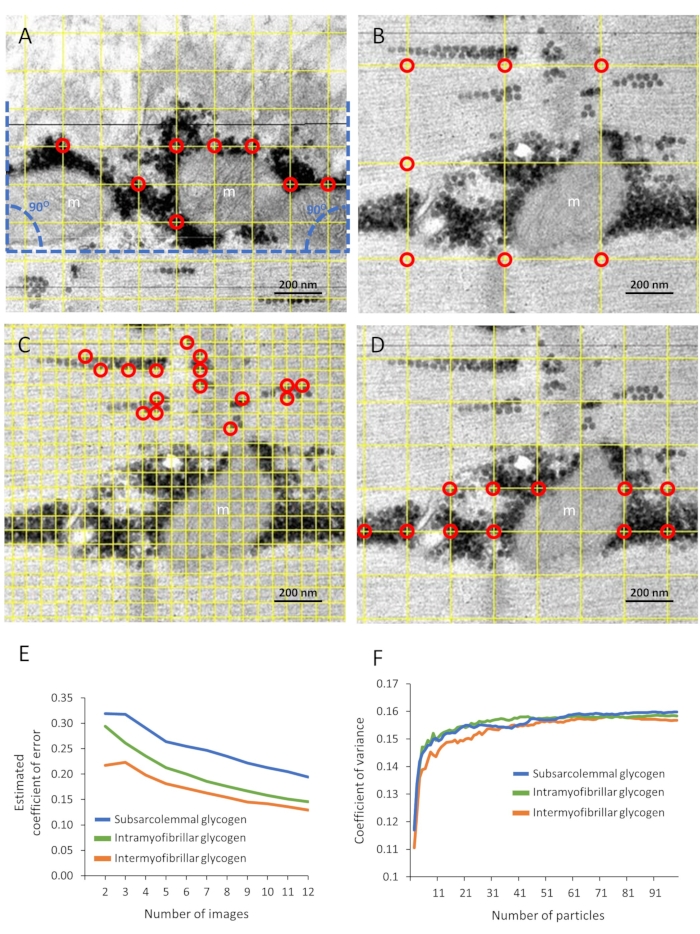
Figure 2: Glycogen analyses. (A) Subsarcolemmal glycogen volume per surface area is estimated by point counting using a grid size of 180 nm x 180 nm within a region defined by the length of the outermost myofibril and the subsarcolemmal region perpendicular to this length (blue dotted lines). (B) The myofibrillar volume fraction is estimated by point counting using a grid size of 400 nm x 400 nm. (C) The volume fraction of intramyofibrillar glycogen is estimated by point counting using a grid size of 60 nm x 60 nm. (D) The volume fraction of intermyofibrillar glycogen is estimated by point counting using a grid size of 180 nm x 180 nm. In A-D, the red circles indicate hits (a cross that hits a glycogen particle). (E) The estimated coefficient of error for a stereological ratio estimate for 2 to 12 analyzed images. The coefficient of error is estimated based on the number of counts and therefore varies between samples based on the glycogen concentration. It is often relatively low when the glycogen content is high and vice versa. (F) The coefficient of variation of glycogen particle diameter after measuring 2-99 particles.

Divulgazioni

The authors have nothing to disclose.

Materials

1,2-Propylene oxide Merck 75-56-9
Embedding 812 resin medium kit Taab T031
Glutaraldehyde solution 25% Merck 1.04239.0250
ITEM Olympus Imaging software
Leica EM AC20 Leica Automatic contrasting system
OSIS Veleta digital camera Olympus
Osmium tetroxide 4% solution Polysciences 0972A
Philips CM 100 Transmission EM Philips
Potassium hexacyanoferrate (II) trihydrate Sigma-Aldrich 455989-245G
Sodium cacodylatbuffer 0.2 M ph 7.4 Ampliqon.com AMPQ40989.0500
Ultra-microtome Leica UC7 Leica
Ultrostain lead citrate 3%, stabilized solution Leica 16707235
Uranyl acetate dihydrate Polysciences 6159-44-0

Tags

Play Video

Citazione di questo articolo
Transmission Electron Microscopy to Quantify Glycogen Distribution in Human Skeletal Muscles. J. Vis. Exp. (Pending Publication), e21462, doi: (2023).

View Video