1. Preparation of substrates/cells for nanoindentation measurements
- Follow the steps given in the Supplementary Protocol for preparation of PAAm hydrogels/cells for nanoindentation experiments. The procedure is summarized in Figure 2.
NOTE: PAAm hydrogels have been chosen as they are the most common hydrogels used within the field of mechanobiology. However, the protocol is equally applicable to any type of hydrogel25 (see Discussion, modifications of the method).
2. Starting up the device, probe choice, and probe calibration
- Follow the steps given in the Supplementary Protocol for starting up the device. For technical details on the operation of optical fiber ferrule-top nanoindenters, check these references17,18.
- Select the nanoindentation probe as described below.
NOTE: All commercially available probes such as the ones used in this protocol are equipped with a spherical tip (Figure 3A). Therefore, the choice narrows down to two variables: cantilever's stiffness and tip radius (Figure 3B).- Choose a cantilever's stiffness (k in N/m) that matches the expected sample stiffness for best results15 (see Figure 3C and Discussion, critical steps in the protocol). For cells, select a probe with k in the range 0.01-0.09 N/m. For hydrogels, select a probe with k in the range 0.1-0.9 N/m, which yields optimal results for gels with expected E between a few kPa and 100 kPa (see Representative Results).
- Choose the tip radius (R in μm) according to the desired spatial resolution of the indentation process. For small cells such as Human Embryonic Kidney 293T (HEK293T) cells (average diameter of ~10-15 μm26) select a sphere with R = 3 μm. For hydrogels, select a sphere with R = 10-250 μm to probe the biomaterial's mechanical properties over a large contact area and avoid local heterogeneities.
- Consult Figure 3C and any additional manufacturer's guidelines to select the appropriate probe.
- Once the probe has been selected, follow the steps in the Supplementary Protocol to mount it on the nanoindenter.
3. Probe calibration
NOTE: The following steps are specific to ferrule-top nanoindentation devices based on optical fiber sensing technology, and they are detailed for software version 3.4.1. For other nanoindentation devices, follow the steps recommended by the device manufacturer.
- On the software's main window, click on Initialize. A calibration menu will appear. Enter the probe details (can be found on the side of the probe's box; k in N/m, R in µm, and the calibration factor in air) in the input boxes.
- Prepare the calibration dish: a thick glass Petri dish with a flat bottom (see Discussion, critical steps in the protocol). Fill the dish with the same medium as the sample dish (this can also be air). Match the temperature of the medium with that of the sample.
- Place the calibration dish under the probe. If required, slide out the probe from the nanoindenter's arm holder and hold it in one hand to make space for placement of the calibration dish. Slide back the probe into place.
- Perform the next two steps for calibration in liquid. If measuring in air, use the provided polytetrafluoroethylene substrate for calibration and skip to step 5.
- Prewet the probe with a drop of 70% ethanol using a Pasteur pipette with the end of the pipette in light contact with the glass ferrule, for the drop to slide over the cantilever and spherical tip27 (see Discussion, critical steps in the protocol).
- Manually slide the nanoindenter's arm downwards until the probe is fully submerged, but still far away from the bottom of the Petri dish. If required, add more medium to the calibration dish. Wait 5 min so that equilibrium conditions are reached in the liquid.
- In the software's Initialize menu, click on Scan Wavelength. The interferometer’s screen will show a progress bar and the Live Signal window on the computer’s software will display the pattern shown in Figure S1A, left. To check whether the optical scan was successful, navigate to the Wavelength Scan panel on the interferometer box. If successful, a sine wave should be visible (Figure 1A, right). See Discussion (troubleshooting of the method) if an error appears.
- In the Initialize menu, click on Find Surface, which will progressively lower the probe until a set threshold in the cantilever's bending is reached. The probe stops moving when contact with the glass Petri dish is made.
- Check whether the probe is in contact with the surface. Move the probe down by 1 µm using the y downwards arrow button on the software's main window. Observe the green signal (cantilever's deflection) in the Live Window of the software for changes in the baseline with each step, when the cantilever is in contact with the substrate (Figure S1B). If there is no change, the cantilever is not in contact (see next step).
- Increase the Threshold value in the Options menu under the Find Surface tab from its default value of 0.01 by a step of 0.01 at a time and repeat the Find Surface step until in contact. Alternatively, bring down the probe to contact in small 1 µm steps until the green baseline starts shifting at each downwards step.
NOTE: For the softest cantilevers (k = 0.025 Nm-1), increase the Threshold value in the Options menu under the Find Surface tab a priori of performing step 6. Start from a threshold value of 0.06 or 0.07 and increase it up to 0.1 if necessary. This is because environmental noise will likely cause the cantilever to bend above the threshold prior to contact. For soft probes, decreasing the Approach Speed (μm/s) in the same menu also improves the procedure. - In the Initialize menu, click on Calibrate.
- Check the Live Signal window of the software and make sure that both piezo's displacement and cantilever's deflection signals move up at the same time (Figure S1C).
- If there is a mismatch in time, the probe is not fully in contact with the glass. Move down the probe at steps of 1 µm until the baseline of the cantilever signal changes (see step 7) and repeat step 9.
- If the cantilever signal does not change at all during the Calibrate step, then the probe is far from the surface. Increase the contact threshold iteratively (see step 8) until the surface is found correctly and repeat calibration from the beginning starting with the wavelength scan.
- When the calibration is complete, check the old and new calibration factors on the pop-up window displayed. If the new calibration factor is in the correct range, click on Use New Factor. If calibration fails, and the new factor is either NaN or is not in the expected range, see Discussion (troubleshooting of the method) for resolution.
NOTE: The new factor should be ~n times lower than the one provided on the probe's box if the calibration was performed in a liquid medium with refractive index n (n = 1.33 for water). If calibration was performed in air, then the new and old calibration factors should be approximately equal. - Check whether the demodulation circle has been correctly calibrated as follows. Navigate to the Demodulation tab on the interferometer desktop. Gently tap on the optical table or on the nanoindenter to induce enough noise. A white circle made up of discrete data points should approximately cover the red circle (Figure S1D).
- If the white circle does not overlap with the red circle, or a warning appears on the interferometer's display, the demodulation circle needs recalibration. This can be done in two ways as described below.
- Continuously tap on the body of the nanoindenter to induce one full circle of noise and press the Calibrate button on the interferometer.
- Enter in contact with the glass substrate and press Calibrate from the Initialize menu of the software's main window. Do not save the calibration factor. At this point, check again and make sure the white circle overlaps with the red circle.
NOTE: If the signal is not just slightly displaced from the demodulation circle but rather became very small or is not visible at all, it means that the cantilever is stuck to the optical fiber. Follow the troubleshooting advice for this problem (see Discussion, troubleshooting of the method) and repeat either steps 13.1 or 13.2. Once the cantilever gets back to its horizontal position (Figure 3A), the signal will recover to the demodulation circle.
- Verify the calibration by performing an indentation on the glass substrate directly after the calibration as described below.
- Load or make an experiment file by clicking on Configure Experiment and add a Find Surface step and Indentation step. For the indentation step, use the default displacement mode settings and change the maximum displacement to the calibration distance (3,000 nm) to displace the probe against the stiff substrate.
- Click on Run Experiment and check the demodulation circle in the interferometer window. Check the white signal and make sure it is on top of the red circle during indentation.
- Check the results on the software's main window in the Time Data graph, and make sure the piezo's displacement (blue line) is equal to the cantilever's deflection (green line) as the indentation starts in contact and no material deformation is expected. If the signals are not parallel, see Discussion (troubleshooting of the method).
- Change the local path in the calibration menu by setting the Calibration Save Path to an appropriate directory.
- When the probe has been successfully calibrated, move the piezo up by 500 μm.
4. Measuring the Young's Modulus of soft materials
- Nanoindentation of hydrogels
- Load the Petri dish containing the sample(s) on the microscope's stage and manually move the nanoindenter's probe to a desired x-y position above the sample.
- Manually slide the probe in solution, taking care to leave 1-2 mm between the probe and the sample's surface at this stage. Wait 5 min for the probe to equilibrate in the medium.
- Focus the z plane of the optical microscope so that the probe is clearly visible.
- Perform a single indentation to tune the experimental parameters as described below.
- Configure a new experiment in the software's main window. Click on Configure Experiment, which will open a new window. Add a Find Surface step. All parameters of the Find Surface step can be changed in the Options menu of the software if required.
NOTE: The Find Surface will lower the probe until the surface is found, and then it will retract the probe to a distance defined by Z Above Surface (µm), above the sample's surface. If the selected cantilever is too stiff for the sample or the sample is sticky, after the step the probe is likely to still be in contact with the sample, which will result in a curve without a baseline (Figure 4C). To solve this problem, increase the Z Above Surface (µm). - Add an Indentation step. Select the Profile tab and click on Displacement Control. Leave the default indentation profile.
- Click on Run Experiment on the main software window. This will find the surface and perform a single indentation.If the single indentation does not look as expected, adjust the experimental parameters as outlined in Figure 4 and Discussion (troubleshooting of the method).
- Configure a new experiment in the software's main window. Click on Configure Experiment, which will open a new window. Add a Find Surface step. All parameters of the Find Surface step can be changed in the Options menu of the software if required.
- Once the indentation looks as desired, configure the matrix scan so that a sufficient area of the sample will be indented. Click on Configure Experiment, add a Find Surface step with the previously determined experimental parameters and add a Matrix Scan step.
- For flat hydrogels, configure a matrix scan containing 50-100 points (i.e., 5 x 10 or 10 x 10 in x and y) spaced at 10-100 µm (i.e., dx = dy = 10-100 µm). Click on Use Stage Position to start the matrix scan from the current stage position. Make sure the Auto Find Surface box is ticked to find the surface at each indentation using the set experimental parameters.
- To avoid oversampling, set the step size to at least twice the contact radius (
 , where δ is the indentation depth).
 - Set up the matrix scan profile in displacement control. Ensure that the profile does not violate the assumptions of the Hertz model (see Discussion, critical steps in the protocol).
- Leave the number of segments to 5, which is the default value, and use the default displacement profile. If necessary, change the displacement profile in terms of maximum displacement and time for each sloped segment, which will affect the maximum indentation depth and the strain rate, respectively. Do not exceed strain rates > 10 μm/s (see Discussion, limitations of the method).
- Enter a value for the approach speed, which determines how fast the probe is displaced toward the sample before contact. Match the retraction speed to the approach speed (see note below).
NOTE: For soft cantilevers and noisy environments, an approach speed of 1,000-2,000 nm/s is recommended. For stiffer cantilevers and controlled environments, this can be increased. - Save the configured experiment in the desired Experiment Path and select a directory where the data will be saved in the Save Path, in the General tab of the Configure Experiment window. Click on Run Experiment.
- To avoid oversampling, set the step size to at least twice the contact radius (
- Once the matrix scan is completed, raise the probe by 200-500 µm and move the probe to a different area of the sample sufficiently far away from the first area.
- Repeat the experiment at least two times so that sufficient data is acquired on each sample (i.e., at least two matrix scans per sample, containing 50-100 curves each).
- Nanoindentation of cells
- Load the sample on the microscope as described above.
- For single-cell indentation, focus the z plane so that both cells and probe are visible at 20x or 40x magnification, depending on cell size and spreading.
- Move the probe above the cell to be indented.
- Configure a new experiment in the software's main window. Click on Configure Experiment, which will open a new window. Add a Find Surface and Indentation step with default parameters in displacement mode.
- Click on Run Experiment, which will find the surface and perform a single indentation. Check whether the indentation was successful. If the curve does not look as expected, adjust the experimental parameters (see Figure 4 and Discussion, troubleshooting of the method).
- If the indentation was successful, add a matrix scan to the experiment. Follow the steps given for hydrogels' nanoindentation experiments; configure the matrix scan so that the step size allows for a small area of the cell to be indented; 25 points spaced at 0.5-5 µm for HEK293T cells.
- Depending on the cell size, adapt the matrix scan to ensure the tip does not indent outside the cell limit, i.e., doing a different map geometry or probing fewer points.
- Click on Run Experiment and wait for it to be completed.
- Once the matrix scan is completed, raise the probe out of contact (50 µm in the z plane).
- Move the probe above a new cell and repeat the process (see Discussion, critical steps in the protocol).
- Cleaning the probe and switching off the instrument
- Follow the steps given in the Supplementary Protocol to clean the probe and switch off the nanoindentation device.
5. Data analysis
- Downloading and installing the software
- Follow the steps given in the Supplementary Protocol to download and install the software for data analysis28,29.
- Screening F-z curves and production of cleaned data set in JSON format
- Launch prepare.py from the command line on the lab computer as outlined in steps 2 to 3.
- If using a Windows computer, hold the shift key while right-clicking on the NanoPrepare folder and click on Open PowerShell Window Here. Type the python prepare.py command and press the Enter key. A GUI will pop up on your screen (Figure S2).
- If using a MacOS computer, right-click on the NanoPrepare folder and click on New Terminal at Folder. Type the python3 prepare.py command and press the Enter key, which will launch the GUI (Figure S2).
- Select the O11NEW data format from the drop-down list. If data is not loaded correctly, then relaunch the GUI and select O11OLD.
NOTE: The O11NEW format works for data obtained using ferrule-top optical fiber sensing nanoindentation devices with software version 3.4.1. This format will also work for previous software versions, at least those belonging to nanoindenters installed in 2019-2020. - Click on Load Folder. Select a folder containing the data to be analyzed-single matrix scan or multiple matrix scans. The top graph (Raw Curves) will be populated with the uploaded data set. To visualize a specific curve, click on it. This will highlight it in green and show it on the bottom graph (Current Curve).
- Clean the data set using the tabs present on the right part of the GUI as outlined below.
- Use the Segment button to select the correct segment to be analyzed, which is the forward segment of F-z curves. The specific number depends on the number of segments selected in the nanoindentation software when performing experiments.
- Use the Crop 50 nm button to crop the curves by 50 nm at the extreme left (if L is ticked), right (if R is ticked), or both sides (if both R and L are ticked). Click this button several times to crop as much as is required. Use this to remove artifacts present at the start/end of F-z curves.
- Inspect the Cantilever tab for the spring constant, tip geometry, and tip radius. Inspect the tab to ensure that the metadata has been read correctly.
- Use the Screening tab to set a force threshold that will discard all the curves that did not reach the given force. Discarded curves will be highlighted in red.
- Use the Manual Toggle button to manually remove curves that have not been correctly acquired. Remove any curves by clicking on the specific curve and selecting OUT, which will highlight the curve in red.
- Click on Save JSON. Enter an appropriate name for the cleaned data set, which is a single JSON file. Send the JSON file to the computer where the NanoAnalysis software was installed.
6. Formal data analysis
- Launch the nano.py file from the command line by navigating to the NanoAnalysis folder and launching a terminal as previously explained. Type the python nano.py or python3 nano.py command (depending on the operating system) and press the Enter key. A GUI will pop up on your screen (Figure S3).
- On the top left of the GUI, click on Load Experiment and select the JSON file. This will populate the file list and the Raw Curves graph showing the data set in terms of F-z curves. Both F and z axes are shown relative to the CP coordinates, which are computed in the background when loading the dataset (see the following note). In the Stats box, check the values of the three parameters: Nactivated, N failed, and Nexcluded.
NOTE: Nactivated represents the number of curves that will be analyzed in the subsequent Hertz/elasticity spectra analysis and appear in black in the Raw Curves graph. Nfailed represents the number of curves on which a reliable CP could not be found and appear in blue in the graph. These curves will automatically be discarded in the subsequent analysis. Upon opening the software, some curves may be automatically moved to the failed set. This is because the CP is calculated upon opening the software with the default Threshold algorithm (see below). Nexcluded represents the curves that are manually selected to be excluded from the analysis and will appear in red in the graph (see below). - Check whether the number of failed, excluded, and activated curves is reasonable. Check the Raw Curves graph to visualize the curves.
- To visualize a specific curve in more detail, click on it. This will highlight it in green and show it on the Current Curve graph. Once a single curve has been selected, the R and k parameters (which must be the same for all curves) will be populated in the Stats box of the GUI.
- Change the status of a given curve using the Toggle box. Click on the specific curve you want to change the status of, and then click on either Activated, Failed, or Excluded. The count in the Stats box is automatically updated.
NOTE: To change the view of the data set in the Raw Curves graph use the View box. Click on Tutti to show all curves (i.e., activated, failed, and excluded in the respective colors). Click on Failed to show the activated and the failed curves and click on Activated to only show the activated curves. To reset the status of all curves between activated and excluded, click on Activated or Excluded in the Reset box. - Once the dataset has been further cleaned, follow the data analysis pipeline outlined below.
- Filter any noise present in the curves using the filters implemented in the GUI (Filtering Box), namely, a custom filter called Prominency filter, the Savitzky Golay30,31 (SAVGOL) filter, and a smoothing filter based on computing the median of the data in a given window (median filter). See Discussion (critical steps in the protocol) for details on filters.
- Inspect the filtered curves in the Current Curve graph. The filtered curve is shown in black whereas the non-filtered version of the curve is shown in green.
NOTE: It is advised to filter the data as little as possible to preserve features of the original signal. Over filtering may smooth out any differences present in the data. Working with the prominency filter activated is enough for the Hertz analysis of nanoindentation data. If the data is particularly noisy, then a SAVGOL or median filters may be additionally applied. - Select an algorithm to find the CP. In the Contact Point box, choose one of a series of numerical procedures that have been implemented in the software, namely, the Goodness of Fit (GoF)32, Ratio of Variances (RoV)32, Second derivative33, or Threshold33. See Discussion, critical steps in the protocol for details on the algorithms.
NOTE: The CP is the point at which the probe comes into contact with the material and needs to be identified in order to convert F-z data into F-δ data (for soft materials, δ is finite and needs to be calculated). The selected algorithm will be applied to all active curves of the data set, and curves where the algorithm fails to locate the CP robustly will be moved to the failed set. - Adjust the algorithm's parameters to suit your dataset so that the CP is located correctly as detailed in the Discussion, critical steps in the protocol.To view where the CP has been found on a single curve, select the curve by clicking on it and click on Inspect. Check the pop-up window that appears to identify where the CP has been located.
- Check whether the red line that appears, which is the parameter the algorithm computed in the selected region of interest, has a maximum or minimum value that corresponds to the location of the CP (e.g., for the GoF, the parameter is the R2). Repeat this process for all curves if needed.
NOTE: The axes of the pop-up are in absolute coordinates so that the location of the CP can be shown. Conversely, the axes of the Raw Curves and Current Curve graph are shown relative to the CP, i.e., the location of the CP is (0,0). - Click on Hertz Analysis. This will generate three graphs described below.
- Check individual F-δ curves in the dataset together with the average Hertz fit (red dashed line). Adjust the indentation in nm up to which the Hertz model is fitted in the Risultati box under Max Indentation (nm). Set it to a maximum of ~10% of R for the Hertz model to be valid (see Discussion, critical steps in the protocol).
- Check the average F-δ curve with error band showing one standard deviation (SD) together with the average Hertz fit (red dashed line). Visualize the average Hertz fit on the Raw Curves graph for reference and the Hertz fit for each curve on the Current Curve.
- Check the scatter plot of E originating from fitting the Hertz model to each individual curve.
- Click on either the file name, F-z curve, F-δ curve, or a point on the scatter plot to highlight the curve in each plot. If a data point in the scatter plot appears to lie outside the distribution of the data, click on it and inspect the curve to which it belongs. Verify that the CP has been located correctly by clicking on the Inspect button. Exclude the curve from the analysis if necessary.
- Inspect the Risultati box for the computed mean E and its SD (Eγ ± σ) and make sure they are reasonable for the given experiment.
- In the Save box, click on Hertz. In the pop-up window, enter file name and directory. Once done, click on Save. A .tsv file will be created. Open the .tsv file in any additional software of preference and use the values for statistical analysis and further plotting.
NOTE: The file contains the E obtained from each curve and the mean E and its SD. Additionally, the file contains metadata associated with the analysis, including the number of curves analyzed, R, k, and the maximum indentation used for the Hertz model. - This step is optional. Click on Average F-Ind to export the average force and the average indentation, together with one SD in the force.
- For cell nanoindentation data, click on Elasticity Spectra Analysis (see Representative Results and Discussion). Inspect the two plots produced, namely, E as a function of the indentation depth (E(δ)) for each curve, and the average E(δ) with error band showing one SD (solid red line and shaded area) fitted by a model (black dashed line), which allows to estimate the cell's actin cortex's Young's modulus, the cell's bulk Young's modulus, and the actin cortex's thickness. Additionally, check the average E(δ) in the top graph in red.
- Make sure the Interpolate box is checked, which ensures the derivative needed to perform the elasticity spectra analysis is computed on the interpolated signal (see Representative Results).
- Inspect the Risultati box, reporting the cortex's Young's modulus (E0 ± σ), the cell's bulk Young's modulus (Eb ± σ), and the cortex thickness (d0 ± σ).
NOTE: The average elasticity spectra may appear noisy at first, with prominent sinusoidal oscillations. As a result, equation (3) may not be fitted correctly. If this is the case, iteratively increasing the window length of the smoothing SAVGOL filter34 solves this issue. - Once the analysis is finished, click on ES in the Save box. This will export a .tsv file in the specified directory, containing the average elasticity as a function of the average indentation depth and contact radius, the metadata associated with the experiment (see above), and the estimated model parameters explained above. Finally, the average elasticity disregarding the dependency on δ and its SD, are also reported.
- Close the software and input the saved results in any other software of preference to further plot the data and perform statistical analysis.
- This step is optional: Export graphs from the GUI by right-clicking on the graph and selecting Export. Export the graph in .svg, so that parameters such as font, font size, line style, etc. can be edited in another software of choice.
NOTE:Custom CP algorithms and filters can be programmed and added to the already existing ones. See Supplementary Note 1 for details.
Following the protocol, a set of F-z curves is obtained. The dataset will most likely contain good curves, and curves to be discarded before continuing with the analysis. In general, curves should be discarded if their shape is different from the one shown in Figure 4A. Figure 5AI shows a dataset of ~100 curves obtained on a soft PAAm hydrogel of expected E 0.8 KPa35 uploaded in the NanoPrepare GUI. Most curves present a clear, flat baseline, a transition region, and a sloped region that is proportional to the apparent stiffness of the material13. However, a minority of curves show alterations from the shape shown in Figure 4A, such as the absence of a baseline, missed contact, or a sloped baseline. These curves can be easily removed from the dataset using NanoPrepare (Figure 5AII, red curves), and a clean dataset saved in the standard JSON format (Figure 5AIII). The clean dataset is uploaded in NanoAnalysis (Figure 5BIV), which has been designed so that it batch processes all curves. This means each step of the workflow is applied to the whole dataset. After being uploaded, curves can be filtered to remove random noise using one or more filters described in the Discussion, critical steps in the protocol (Figure 5BV). The CP is then located using one of the algorithms implemented in the software and detailed in the Discussion, critical steps in the protocol (Figure 5BVI). Once the CP has been identified, F-z data is converted into F-δ data. Because the software has been designed to primarily analyze data from ferrule-top nanoindentation devices based on optical fiber sensing, which use probes having a spherical tip, the Hertz analysis is based on the Hertz model approximating the contact between a sphere of radius R and an infinitely extended linear elastic homogeneous isotropic (LEHI) half space13:
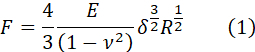
where F is the force, δ is the indentation, E is Young's Modulus, and ν is the Poisson's ratio, taken as 0.5 assuming incompressibility. By fitting F-δ curves with equation (1), E can be therefore estimated (see Discussion-critical steps in the protocol-for assumptions of the Hertz model) (Figure 5BVII).
In addition to the Hertz analysis, the software can perform a more advanced analysis, namely, the elasticity spectra, which is particularly useful for cell nanoindentation data; and can also be used as a tool to estimate the influence of the underlying substrate on the mechanical properties obtained via the Hertz model. Below, the approach is briefly summarized. Full details can be found in the original publication24.
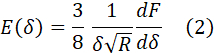
Starting from the Oliver-Pharr model36, which describes the indentation of an axisymmetric punch of arbitrary geometry and an elastic half space, one can derive E(δ) for the specific case of a spherical indenter. Taking ν as 0.5, E(δ) has the form24:
Computing E(δ) for each F-δ curve using equation (2) yields a set of curves, namely, the elasticity spectra (ES). By taking the average of all curves in the data set, the average ES is obtained (Figure 5BVIII, red solid line). The average ES is a useful tool because it provides information on how E varies with δ in the dataset. In the specific case of cell nanoindentation experiments, the thickness of the cell is not known a priori, which means that choosing an appropriate fitting range for the Hertz analysis is somewhat arbitrary. By using the average ES, substrate effects on the apparent E(δ) become evident, which means the tool can be used to select an appropriate fitting range, corresponding to the point where E(δ) starts increasing after its decay. Further, it has been previously demonstrated and computationally and experimentally validated that a simple bilayer model is effective in the estimation of the actin cortex's thickness (d0), the actin cortex's Young's modulus (E0), and the cell's bulk Young's modulus (Eb)24. The model describes the cell as a bilayer, with an outermost layer of thickness d0 and modulus E0, and an inner layer of infinite thickness with elastic modulus Eb<E0:
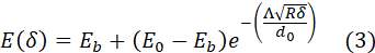
where R is the tip's radius and Λ is a phenomenological parameter, which was determined to be 1.74 from finite element analysis simulations24. This procedure has been implemented in the NanoAnalysis software, which allows to fit the average ES with equation (3) to obtain an estimate of E0, Eb, and d0 (Figure 5BVIII, black dashed line). For full methodological details, refer to the original publication24.
To demonstrate the viability of the protocol, the elasticity of PAAm hydrogels of known E (measured by AFM)35 were prepared and tested using the procedure suggested in Part 1 of the protocol. For each gel, two stiffness maps in two different areas of the sample were acquired using a commercial ferrule-top nanoindenter equipped with a tip having R = 52 µm and k = 0.46 N/m. Each map consisted of 50 indentations performed in displacement control, and the step size in x and y was set to 20 µm to avoid oversampling. Figure 6A shows the average F-δ curve together with the average Hertz model for a soft PAAm hydrogel (expected E 0.8 kPa) and a stiff PAAm hydrogel (expected E 8 kPa)35. By performing the Hertz analysis through the NanoAnalysis software and plotting individual values of E, the expected E was retrieved for both hydrogels (Figure 6B).
Further, nanoindentation experiments on HEK293T cells were performed. Six individual cells were indented by performing a matrix scan with x and y step size set to 0.5 µm on each cell and acquiring a minimum of 25 curves on each cell. This resulted in the analyzed dataset containing ~200 curves. The selected probe had R = 3.5 µm and k =0.02 N/m.
Figure 7A shows the average Hertz curve and the corresponding average Hertz model, plotted using the mean E obtained from fitting equation (1) to each individual curve in NanoAnalysis up to an indentation of 200 nm. E was found to be 915 ± 633 Pa (mean ± SD), which is in accordance with values reported in the literature24. Despite its wide use, the Hertz model does not fully capture the evolution of the force with increasing indentation depth for cell nanoindentation experiments (Figure 7A). Because of this, the ES is a particularly suitable tool to study the mechanical properties of single cells.
Figure 7B shows the average ES, together with equation (3) fitted up to an indentation of 200 nm. The average ES starts increasing at an indentation depth of ~200 nm, which indicates the contribution of the substrate to the probed apparent E (Figure S4). Because of this, 200 nm was chosen as the fitting range for both the Hertz model (Figure 7A) and the bilayer model (Figure 7B). Fitting equation (3) to the average ES allowed to extract important information, which would otherwise remain inaccessible from simple nanoindentation experiments analyzed using the Hertz model. Specifically, the actin cortex's modulus E0 was estimated to be 5.794 ± 0.095 kPa, the actin cortex's thickness d0 was found to be 311 ± 3 nm and the bulk modulus Eb was found to be 0.539 ± 0.002 kPa (mean ± SD). All values are in accordance with previous experiments performed using AFM on the same cell type24, and with values that have been reported in the literature37,38. Specifically, the actin cortex is expected to be between 300-400 nm for adherent cells37, and up to 10 times stiffer than the bulk of the cell38.
Regardless of the bilayer model, a direct comparison between results obtained with the standard Hertz model and the ES approach is given in Figure 7C, which reveals overlapping distributions with comparable means.
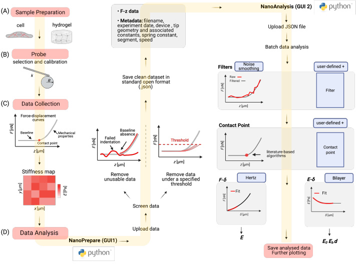
Figure 1: Protocol overview. The protocol consists of the following parts: (A) Part 1: Preparing the sample (either hydrogels or cells) for nanoindentation experiments. (B) Part 2: Choosing the right probe and calibrating the probe. (C) Part 3: Performing nanoindentation experiments by acquiring stiffness maps on the sample. (D) Part 4: Analyzing the data, which consists of i) cleaning the acquired dataset through the first GUI (NanoPrepare) and saving the cleaned dataset and associated metadata as a standard JSON file; and ii) analyzing the cleaned dataset in the second GUI (NanoAnalysis), which consists of data filtering, CP identification, and model fitting to estimate Young's modulus E of the sample. Results are saved for further plotting and statistical analysis, which can be performed in any software of choice. Created with Biorender.com. Please click here to view a larger version of this figure.
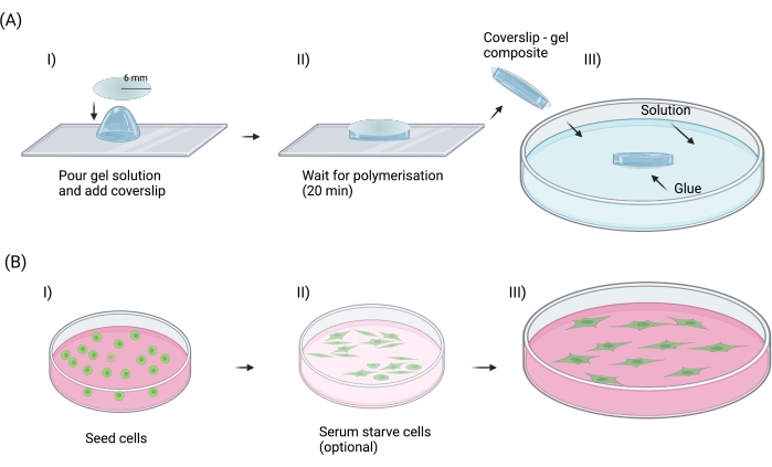
Figure 2: Sample preparation. (A) Steps suggested to prepare flat PAAm hydrogels for nanoindentation experiments. These are: I) pouring the hydrogel solution onto a hydrophobic glass slide and covering it with a silanized coverslip; II) waiting for 20 min for polymerization to occur and peeling off the coverslip-gel composite from the glass slide; and III) attaching the coverslip-gel composite to a Petri dish and adding appropriate solution (purified water in the context of this protocol) for nanoindentation experiments. The same rationale can be adapted and applied to any other type of hydrogel. (B) Steps suggested to prepare cells for nanoindentation experiments. These are: I) seeding cells and waiting for cell adhesion; II) serum starving the cells to synch the cell population in terms of the cell cycle (optional); and III) waiting for cells to be in an adhered state at desired confluency before starting nanoindentation experiments. Created with Biorender.com. Please click here to view a larger version of this figure.
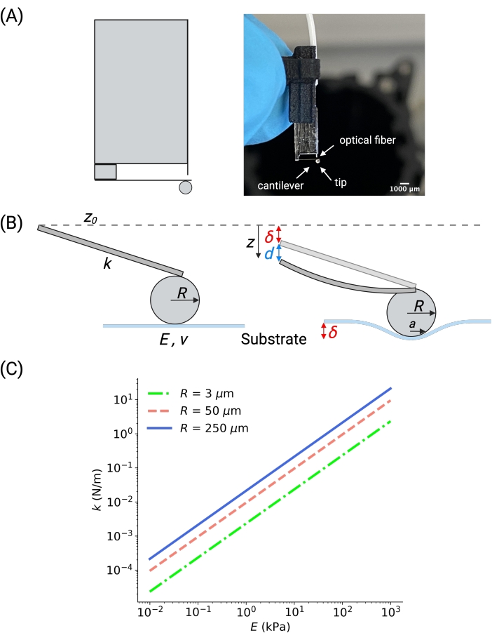
Figure 3: Nanoindentation probe overview and selection. (A) Schematic of ferrule-top probe (left) and picture of a ferrule-top probe with the spherical tip of radius 250 µm (right). All components are labeled in the photo. (B) Enlarged schematic of the cantilever and the spherical tip. The cantilever is treated as a Hookean spring of elastic constant k (shown at an angle for representation purposes). The tip is defined by its radius, R. When the sample is indented, the probe is displaced by an amount z from its reference position z0, which results in the cantilever bending d from its reference bending d0. A force of F = k (d – d0) is applied to the sample, which results in an indentation δ = (z – z0) – (d – d0). (C) Cantilever's stiffness k should be chosen according to the expected elasticity of the substrate. The plot was obtained considering Hertzian contact with an indentation of 1 µm, assuming that the energy is equally shared between the cantilever's bending and the substrate's indentation (i.e., d =δ). The larger the tip radius, the stiffer the cantilever should be to reach the same indentation for a substrate with a given E. Please click here to view a larger version of this figure.
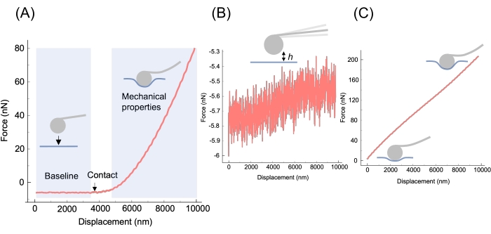
Figure 4: Morphological characteristics of F-z curves. (A) A successful experiment results in the approach segment of an F-z curve having a clear baseline (tip approaching the sample but not in contact); a transition region where the tip first contacts the sample; and a region where the force increases with the displacement, where the tip is progressively indenting the sample. The slope of this region is proportional to the apparent stiffness of the material13, meaning that curves belonging to stiff biomaterials (e.g., highly crosslinked gels) will be steeper than those belonging to softer biomaterials (e.g., weakly crosslinked gels and cells). (B) An approach curve where the tip never entered contact with the sample. See troubleshooting of the method in the Discussion for resolution. (C) An approach curve where the tip started in contact with the sample. See troubleshooting of the method in the Discussion for resolution. The data shown is from an experiment performed on a soft PAAm hydrogel of expected E 0.8 kPa35. Please click here to view a larger version of this figure.

Figure 5: Data analysis workflow using the Python GUIs. (A) An example dataset of F-z curves acquired using a commercially available ferrule-top nanoindenter on a soft PAAm hydrogel (expected E 0.8 kPa35) was uploaded in NanoPrepare. Curves that do not follow the shape described in Figure 4A are excluded from the dataset, and the clean dataset and associated metadata are saved as a standard JSON file. (B) The clean dataset is uploaded in the second GUI (NanoAnalysis) where curves can be filtered by applying one or more filters to remove noise (see Discussion, critical steps in the protocol). Further, a CP algorithm is selected to automatically locate the CP for all curves (see Discussion, critical steps in the protocol). The Hertz analysis is then performed, yielding a F-δ curve for each indentation, which is fitted with the Hertz model to yield a scatter plot of E. The obtained results can be saved for further plotting. For cells, an additional analysis called the elasticity spectra24 can be performed. All graphs shown were directly exported from both NanoPrepare and NanoAnalysis GUIs. Details for each step of the workflow are given in the main text. Please click here to view a larger version of this figure.
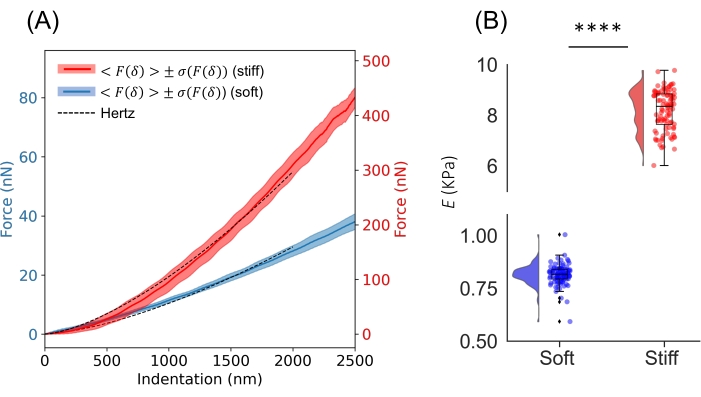
Figure 6: Elasticity of PAAm hydrogels. (A) Average F-δ curve from a set of ~100 curves acquired on a soft PAAm hydrogel (expected E 0.8 kPa35) and a stiff PAAm hydrogel (expected E 8 kPa35). Solid lines show the mean and shaded band shows one SD. The dashed line shows the Hertz model plotted using the average E from the NanoAnalysis software, obtained by fitting the Hertz model to each curve up to a maximum indentation of 2,000 nm (~4% of R, R = 52 µm, k = 0.46 N/m). Curves were smoothed using the prominecy filter with default parameters, and the CP was identified using the RoV algorithm32. (B) Individual values of E obtained from the analysis performed in NanoAnalysis plotted for statistical comparison. The raincloud plot was obtained using the Python module described in reference39. **** p < 0.0001, two-tailed unpaired t-test, α=0.05. Please click here to view a larger version of this figure.
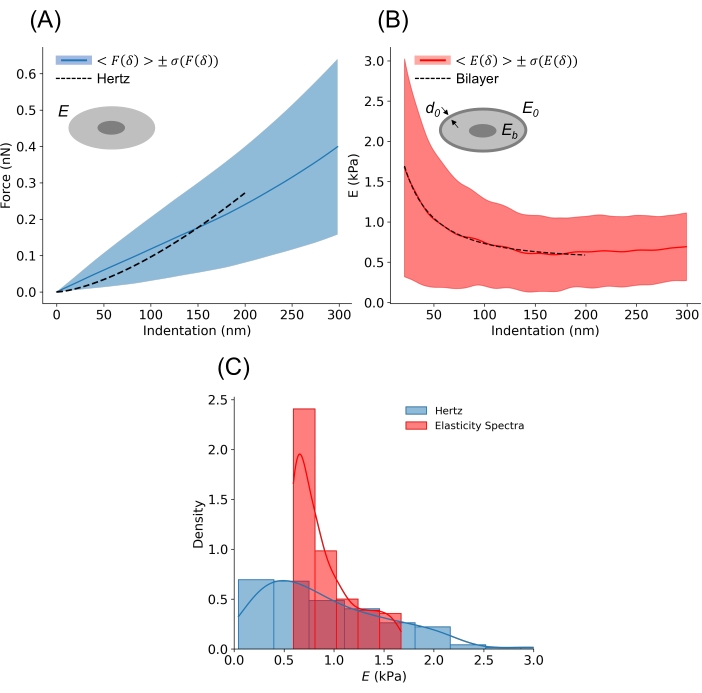
Figure 7: Elasticity of HEK293T cells. (A) Average F-δ curve from a set of ~200 curves acquired on six individual HEK293T cells. The solid blue line shows the mean and the shaded band shows one SD. The dashed line shows the Hertz model plotted using the average E computed using the NanoAnalysis software, obtained by fitting the Hertz model to each curve up to a maximum indentation of 200 nm (~6% of R, R = 3.5 µm, k = 0.02 N/m). Curves were smoothed using the prominecy filter with default parameters and a SAVGOL filter34 with order 3 and window length 80 nm, and the CP was identified using the Threshold algorithm33. Using the Hertz model, the cell is treated as a homogeneous sphere with Young's Modulus E, as schematically shown in the inset (the nucleus is depicted for pictorial purposes). (B) Average elasticity spectra computed on the same data set described in (A). The solid red line shows the mean and the shaded band shows one SD. By fitting a bilayer model to the average elasticity spectra, estimations of E0, Eb, and d0 are computed. For the dataset shown: E0 = 5.79 ± 0.09 kPa, Eb = 0.539 ± 0.002 kPa and d0 = 311 ± 3 nm (mean ± SD). (C) Comparison between the Hertz model and the elasticity spectra approach in terms of E distribution. For the elasticity spectra, the distribution represents the values of E from the average elasticity spectra, regardless of indentation depth (up to a maximum indentation of 200 nm). The continuous lines superimposed on the histograms are Gaussian kernel density estimates of the underlying distributions. E = 915 ± 633 Pa (Hertz) and E = 890 ± 297 Pa (elasticity spectra) (mean ± SD). Please click here to view a larger version of this figure.
Figure S1: Calibration Procedure. (A) Successful wavelength scan. The cantilever's deflection and piezo's displacement signals during the wavelength scan (left). The sinusoidal wave on the interferometer's screen at the end of the wavelength scan (right). (B) Find surface procedure. cantilever's deflection and piezo's displacement signals as the probe is lowered in 1 μm steps after contact with a stiff substrate. (C) Geometrical factor calibration. During indentation of a stiff substrate, the cantilever's deflection follows the cantilever's displacement (green and blue lines, respectively). The indentation should be approximately zero (red line). If the deflection lags the displacement in time (green dashed line), the probe is not fully in contact with the stiff substrate. (D) Demodulation signal. The demodulation signal on the interferometer's screen at the end of the calibration procedure (left) and when tapping on the nanoindenter (right). Please click here to download this File.
Figure S2: NanoPrepare GUI. Screenshots of the NanoPrepare GUI. Details on the functionality of each widget are given in the main Protocol and the Discussion. Please click here to download this File.
Figure S3: NanoAnalysis GUI. Screenshots of the NanoAnalysis GUI. Details on the functionality of each widget are given in the main Protocol and the Discussion. Please click here to download this File.
Supplementary Note 1: Adding custom filters and CP algorithms to the NanoAnalysis software. Please click here to download this File.
Supplementary Protocol. Please click here to download this File.
Figure S4: Depth dependency of average elasticity spectra. The plot shows the average elasticity spectra <E (δ)> (solid red line) together with one SD (σ(E(δ)). After an initial decay, the average elasticity spectra start increasing, which is mainly associated with the effects of the stiff underlying substrate on the probed apparent elastic modulus. The maximum indentation depth used to fit the Hertz model to F–δ curves, and the decay model to the average elasticity spectra should be chosen so that the underlying substrate does not affect the results (Fit range). Please click here to download this File.
