JoVE Educazione Scientific
Mechanical Engineering
È necessario avere un abbonamento a JoVE per visualizzare questo.  Accedi o inizia la tua prova gratuita.
JoVE Educazione Scientific Mechanical Engineering
Jet Impinging on an Inclined Plate
  • 00:06Panoramica
  • 01:39Principles of Jet Impingement
  • 05:40Setup and Calibration
  • 07:25Data Acquisition
  • 08:57Data Analysis
  • 10:04Risultati
  • 11:39Applications
  • 13:02Summary

Jet que inciden sobre una placa inclinada

English

Condividere

Panoramica

Fuente: Ricardo Mejía-Alvarez y Hussam Hikmat Jabbar, Departamento de ingeniería mecánica, Universidad Estatal de Michigan, East Lansing, MI

El objetivo de este experimento es demostrar cómo un fluido ejerce fuerzas sobre las estructuras por la conversión de presión dinámica en presión estática. Para ello, vamos a hacer un chorro plano incidir un plano de la placa y medir la distribución resultante de la presión a lo largo de la placa. La fuerza resultante se calcula mediante la integración del producto entre la distribución de la presión y diferenciales de área adecuadamente definida a lo largo de la superficie de la placa. Este experimento se repetirá para dos ángulos de inclinación de la placa con respecto a la dirección del jet y dos caudales. Cada configuración produce una distribución de presión a lo largo de la placa, que es el resultado de diferentes niveles de conversión de presión dinámica en presión estática en la superficie de la placa.

Para este experimento, la presión se medirá con un transductor de presión de diafragma conectado a una válvula de barrido. La placa en sí tiene pequeñas perforaciones llamados grifos de presión que conectan a la válvula de barrido a través de mangueras. La válvula de barrido envía la presión de estos grifos para el transductor de presión uno a la vez. La presión induce la deformación mecánica sobre el diafragma que el transductor de presión se convierte en tensión. Este voltaje es proporcional a la diferencia de presión entre los dos lados del diafragma.

Principi

Procedura

1. configuración de la instalación Asegúrese de que no hay ningún flujo en la instalación. Establecer los instrumentos según el esquema en la figura 2. Ajustar la placa de ángulo . Registre este valor en la tabla 1. Medir el ancho de boquilla de chorro . Registre este valor en la tabla 1. Medir la duración de la placa L. registro este valor en la tabla 1. A cero el transductor de …

Risultati

Figure 4 shows four sets of results obtained for the plane jet impinging on a plate at two different angles and two different flow rates. In fact, since the low-pressure side of the transducer is opened to the receiver, its readings correspond only to the overpressure , which are in fact the points shown in Figure 4.

Figure 4
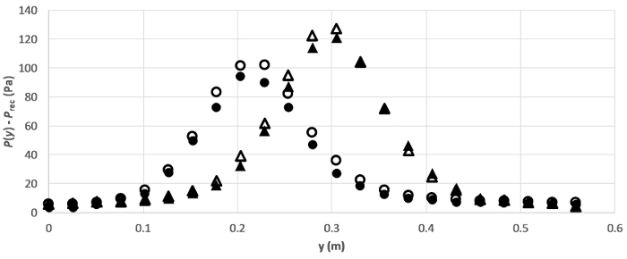
Figure 4. Representative results. Pressure distribution along the plate for two angles and two flow rates. Symbols represent: : , m/s; : , m/s; : , m/s; : , m/s.

According to Figure 4, the profiles for 90o impingement are higher than the ones for 70o impingement. The reason for this behavior is that the stagnation streamline for the former case corresponds to the flow centerline, that is, the streamline for peak velocity and consequently maximum dynamic pressure. While the stagnation streamline moves away from the peak velocity line and bends away from its original path as the impingement angle decreases. This effect is sketched in Figure 1(A), and it is also the reason why the peak pressure in the pressure profile moves away from the center of the plate.

As expected, the maximum pressure decreases with flow rate (closed symbols in figure 4) because there is a general reduction in kinetic energy and hence in dynamic pressure as the flow rate decreases. This maximum pressure is in fact a measure of the stagnation pressure, , previously explained. For the case of the jet impinging the plate at 90o, this is an accurate measure of because the pressure tap coincides with the centerline, ergo the stagnation streamline, of the jet. But as suggested in figure 1a, the stagnation streamline bends away from its original path as the impingement angle decreases. Under this new condition, there is not guarantee that this streamline will exactly coincide with a pressure tap at its impingement location. Hence, the peak pressure observed at impingement angles different than 90o is just an approximation to .

Table 2 shows the results obtained in experimental measurements for two different impinging angles and flow rates.

Table 2. Representative results.

Parameter Run 1 Run 2 Run 3 Run 4
Plate angle (θ) 90o 90o 70o 70o
Digital multi-meter reading (E) 2.44 V 2.33 V 2.44 V 2.28 V
Pressure difference (P_pl-P_rec )    335.95 Pa 320.80 Pa 335.95 Pa 313.92 Pa
Velocity at vena contracta (V_VC) 10.14 m/s 9.91 m/s 10.14 m/s 9.81 m/s
Mass flow rate ((m)) ̇ 0.254 kg/s 0.249 kg/s 0.254 kg/s 0.246 kg/s
Stagnation pressure (P_o ) 127.16 Pa 121.19 Pa 101.78 Pa 94.31 Pa
Load on the plate (F) 16.84 N 16.24 N 14.11 N 12.32 N

Applications and Summary

The experiments featured herein demonstrated the interplay of pressure and velocity to generate loads in objects by means of conversion of dynamic pressure into static pressure. These concepts were demonstrated with a plane jet impinging on a flat plate at two different angles and two different flow rates. The experiments clearly demonstrated that the load is highest at the stagnation point, where all the dynamic pressure is converted into static pressure, and its magnitude decreases as the level of conversion from dynamic to static decreases at positions away from the stagnation point. The angle of incidence has the effect of reducing the total load because it shifts the stagnation pressure from the one coinciding with the centerline (maximum) velocity to a streamline carrying lower levels of dynamic pressure.

These experiments also served the purpose of demonstrating how to determine the total load on the object exposed to the flow by numerically integrating the data obtained from pressure taps. In addition, the reverse conversion of static pressure into dynamic pressure was also used to estimate the velocity and mass flow rate of the jet. In consequence, the interplay of pressure and velocity can be used for flow diagnostics.

A concept that was not explored in the present experiment is velocimetry by Pitot – static probes. These are probes that directly measure the difference between the stagnation and static pressures, which is exactly what was used in equation (3) to determine the velocity at the vena contracta. Note that, at least in the 90o angle plate, the central pressure tap is directly exposed to the stagnation point, making it a Pitot probe. Since the pressure transducer compares the pressure of each pressure tap to the receiver's pressure, the result is a direct measurement of . Upon substitution of this measurement in equation (3), the result is the velocity of a point on the stagnation streamline that is close to the stagnation point but still outside of its radius of influence. This measurement is of limited use in this experiment because the exact location of that point on the stagnation streamline is not known.

As mentioned before, pressure measurements can be used to determine flow velocity. In the application described herein, the change in pressure between the plenum and the receiver were enough to estimate the average velocity at the vena contracta.It was also mentioned that, incidentally, the pressure tap coinciding with the stagnation point is a Pitot tube that could be used in conjunction with a probe sensing the static pressure to determine flow velocity from equation (3) (substituting with and with ). In fact, a single device combining a Pitot probe and a static probe, known as Prandtl tube, might be the most extended diagnostic device in fluids engineering to measure velocity. As shown in figure 5, this probe is composed by two concentric tubes. The inner tube faces the flow to detect the stagnation pressure, and the outer tube has a set of side ports that sense the static pressure. A sensor such as a pressure transducer or a liquid column manometer is used to determine the difference between these two pressures to estimate the velocity from equation (3) (again, substituting with and with ). A probe like this, or a combination of a Pitot and an independent static probe is in fact used in airplanes to determine the velocity of the wind relative to the airplane.

Figure 5
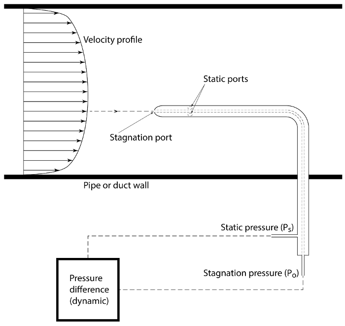
Figure 5. Flow velocimetry. Pitot-static (or Prandtl) probe to determine the velocity distribution based on the dynamic pressure. This probe is traversed across the flow field to determine the velocity at different positions. Please click here to view a larger version of this figure.

Riferimenti

  1. Arnau, A. (ed.). Piezoelectric transducers and applications. Vol. 2004. Heidelberg: Springer, 2004.
  2. Tropea, C., A.L. Yarin, and J.F. Foss. Springer handbook of experimental fluid mechanics. Vol. 1. Springer Science & Business Media, 2007.
  3. White, F. M. Fluid Mechanics, 7th ed., McGraw-Hill, 2009.
  4. Chapra, S.C. and R.P. Canale. Numerical methods for engineers. Vol. 2. New York: McGraw-Hill, 1998.
  5. Buckingham, E. Note on contraction coefficients of jets of gas. Journal of Research,6:765-775, 1931.
  6. Munson, B.R., D.F. Young, T.H. Okiishi. Fundamentals of Fluid Mechanics. 5th ed., Wiley, 2006.
  7. Lienhard V, J.H. and J.H. Lienhard IV. Velocity coefficients for free jets from sharp-edged orifices. ASME Journal of Fluids Engineering, 106:13-17, 1984.

Trascrizione

Jet impingement on solid structures is a widely used process in technological applications, such as material cutting in the manufacturing industry and energy generation from hydraulic sources. Jet impingement consists of releasing a fluid through a nozzle from a high-pressure region to a low-pressure region and striking or impinging the jet upon a structure. During the process of impingement, forces generated by the interplay between pressure and velocity of the flow field are exerted on the object’s surface. For example, in the case of a vertical takeoff and landing or VTOL aircraft, two jets combined produce enough lift to help the aircraft take off vertically without using the runway. Two additional smaller jets issued on each side of the aircraft provides stability. The effects of impingement depend on the jet’s dimensions and speed, the characteristics of the impingement surface, and the distance between the nozzle and surface. When the temperatures of the surface and the jet are significantly different, jet impingement would produce high levels of heat transfer. This video will illustrate how to determine the load exerted by a jet on an object and also how to calculate other parameters of interest for flow diagnostics, such as jet velocity and mass flow rate.

Before delving into the experimental protocol, let’s study the principles behind jet impingement. For a steady incompressible flow of a fluid with zero viscosity, the kinetic energy and pressure potential energy are free to transform into each other along the streamlines. While the sum of the two forms of energy is always constant, this is Bernoulli’s Principle derived from the Principle of Energy Conservation. According to this principle, an increase in speed and in consequence in the kinetic energy of a fluid occurs simultaneous with a decrease in its pressure and potential energy. Such as their sum is always constant. This is Bernoulli’s Equation. Expressed in dimensions of pressure, the term associated with kinetic energy is called dynamic pressure. While the term associated with the pressure potential energy, is called static pressure. The addition of these two terms gives the Bernoulli’s constant, also known as stagnation pressure. Stagnation pressure is defined as the maximum pressure that the flow would reach if brought to a halt by transforming all of its dynamic pressure into static pressure. Now let’s talk about the experimental setup. An air jet exits from a high-pressure plenum through a slit of width W and span L to a lower-pressure receiver where the jet impinges on an inclined plate of angle theta. The intermediate streamline divides the jet in two regions. One deflected upwards and the other one downwards. The dividing streamline stops right at the wall at the stagnation point where the dynamic pressure is converted completely into static pressure. At the stagnation point, the profile of the pressure exerted by the jet on the plate has a maximum value p0. While away from this point, the pressure profile steadily decreases since progressively less dynamic pressure gets converted into static pressure. The pressure profile depends on the impingement angle theta. When theta is 90 degrees, the centerline is also the stagnation line. By decreasing the impingement angle, the stagnation streamline moves away from the centerline of the jet, and in consequence, the peak of the pressure profile gets smaller and shifts towards regions of the plate closer to the jet exit. The total pressure on the surface of the plate exposed to the jet is the result of the addition between the impingement pressure and the static pressure inside the receiver. Since the pressure inside the receiver is homogeneously distributed, the surrounding pressure exerted on both sides of the plate cancels out. In consequence, the net load on the plate is due to the overpressure and it is calculated by integrating over the impingement pressure distribution across the area of the plate. When a fluid is discharged through a slit from a high-pressure region to a low-pressure region, the jet tends to converge to an area called vena contracta. This is the first location after the jet leaves its discharge port in which the streamlines become parallel and consequently the static pressure equals the pressure of the surroundings. Let’s apply the Bernoulli’s equation between the position where the jet exits from the plenum and the position at the vena contracta. Considering the velocity inside the plenum to be negligible, the velocity at the vena contracta can be calculated using the pressure difference between the plenum and the receiver. Finally, knowing the contraction ratio between the slit width and vena contracta, the mass flow rate can be estimated using the jet velocity and area of the vena contracta. In the following sections, we will measure the resulting pressure distribution on the plate and then calculate the total force by integrating the pressure field over the plate’s area.

Before starting the experiment, since opening the door to the receiver while in operation is potentially hazardous and damaging to the facility, make sure that the facility is not in use. If the door to the receiver is open, the facility is not in use. If the door to the receiver is closed, look through the window. If there are no personnel inside, the door is safe to open because the facility can only be started from inside while the door is closed. To begin, set the instruments according to the schematic. Connect the positive port of the pressure transducer to the output of the scanning valve. Make sure the scanning valve is at the home position. Connect the piezometric hoses of the plate to the scanning valve in subsequent order. Remember to start the measurements at the intake next to the output of the scanning valve. First, adjust the plate to the desired angle theta. Second, measure the jet nozzle width. Third, measure the span and height of the plate. Zero the pressure transducer and record the value for the calibration constant. Record all the basic parameters of the experiment in a reference table. First, open the low-pressure port to sense the pressure in the receiver. Then connect the high-pressure point of the transducer marked as positive to the pressure tap of the plenum. Next, start the flow facility. Measure the voltage associated with the pressure difference sensed by the pressure transducer between the plenum and the receiver using the digital multimeter. Calculate this quantity using the calibration constant.

Once the instrument is calibrated and the basic parameters are recorded, you are ready to start data acquisition. First, connect the high-pressure port of the transducer to the common port of the scanning valve. Also hone the scanning valve to start your measurement from the first pressure tap position on the plate. Run Traverse six on your computer, input the conversion factor from volts to pressure, and set the sampling rate to 100 hertz and the total of samples to 500 to get five seconds of data. Next, enter zero in the virtual instrument for the position of first pressure tap and then record the data. The value on the screen is the pressure difference between the pressure tap and the receiver. Step the scanning valve to the next tap position. Introduce the new position in the software knowing that the distance between two consecutive taps is 25.4 millimeters and record the new value of the pressure difference. At the end of the experiment, the software generates a table and a plot of the tap position versus the pressure. Modify the flow rate by changing the position of the flow control plate to close the flow area roughly by half and repeat the pressure measurements. Repeat the measurements for different flow rates and inclination angles and record every time your results in a table. When all of the data has been collected, turn the flow facility off.

Based on the experimental data, several parameters of interest can be obtained. Look at the results table and for each plate angle and flow rate, use the pressure difference between the plenum and receiver to calculate the jet velocity at the vena contracta. From the reference table, take the values for the span L and the slit’s width, and use the speed at the vena contracta previously calculated to estimate the mass flow rate. Then look at the position versus pressure plot generated by Traverse six and read the peak value of the pressure. Introduce the value in the results table. This value is a direct estimation of the stagnation pressure. Now, compute the force impinged on the plate by integrating the pressure distribution over the plate area. In order to do this, use the pressue difference versus position plot and calculate the area under the curve with the Trapezoid Rule or Simpson’s Rule. Introduce the value in the results table.

Begin by plotting on the same graph four sets of results obtained for the plane jet impingement on a plate at two different angles and two different flow rates. Now, compare the pressure profiles for the two different impingement angles and the same flow rate. The pressure profile at 90 degrees is higher than the one for 70 degrees. While the peak for 90-degree impingement is centered, the peak for 70 degrees is shifted toward a lower x value. These results tell you that for a 90-degree impingement angle, the stagnation streamline corresponds to the flow centerline. The centerline is characterized by the peak velocity and, thus, by the maximum dynamic pressure. As the impingement angle decreases, the stagnation streamline moves away from the peak velocity line and bends away from its original path. Next, compare the pressure profiles for the two different flow rates and the same impingement angle. The maximum pressure decreases with the flow rate because there is a reduction in the kinetic energy and hence in the dynamic energy as the flow rate decreases. Look at the results table and compare the values calculated for the load on the plate. The impingement angle has the effect of reducing the total load because it shifts the stagnation pressure from the one coinciding with the centerline velocity to a streamline carrying lower levels of dynamic pressure.

Impinging jets are widely used in many industrial and engineering applications spanning from hydraulics and aeronautics to electronics. The interplay of pressure and velocity can be used for flow diagnostics. A Prandtl or pitot-static probe is composed of two concentric tubes. The inner tube faces the flow to detect the stagnation pressure. While the outer tube has a set of side ports that sense the static pressure. The difference in pressure is detected with an integrated sensor, and this value is used to estimate the velocity. This device is extensively used in fluid engineering. To determine for example, the velocity of the wind relative to the airplane. Soft materials like plastics and wood can be cut with a thin waterjet at high speed. While metals can be cut with water upon adding abrasive particles to the stream. To generate a high-speed jet for cutting purposes, it is necessary to impose high pressure in the flow to be able to accelerate it through a converging nozzle. The high kinetic energy carried by the jet is then converted into dynamic pressure at the surface of the object being cut, exerting a force strong enough to remove material at the impinging surface.

You’ve just watched Jove’s Introduction to Jet Impingement on an Inclined Plate. You should now understand how the interplay between pressure and velocity generates forces on the structures and be able to calculate the impingement forces, flow velocities and mass flow rates. Thanks for watching.

Tags

Cite This
JoVE Science Education Database. JoVE Science Education. Jet Impinging on an Inclined Plate. JoVE, Cambridge, MA, (2023).