Conservation of mass is a well-known physical principle that is used together with the control volume approach for engineering of many mechanical systems. Control volume analysis of mass conservation is particularly useful to estimate flow rates for large-scale hydraulic structures, such as dams, water treatment plants, or water distribution systems. This method is usually applied as an initial step to give the engineer an idea of the dominant mass exchange in a system. An outlet valve, for example, constructed through the face of the dam is routinely used to control the flow of water. Since mass is conserved, the net mass flux through a control surface, and the rate of change of mass inside the enclosed volume must be in balance. This video will illustrate how to apply the control volume method for mass conservation to calibrate a smooth contraction as a flow meter.
General principles of the control volume method for conservation of linear momentum were discussed in our previous video. Here, we illustrate this approach for conservation of mass. Consider the flow passage in the schematic, consisting of a centrifugal fan with the smooth contraction at the intake. How does the control volume analysis for conservation of mass apply to our system? First, let’s take an imaginary closed surface, called Control Surface, to define a control volume containing a region of flow. Next, let’s write the general equation for conservation of mass. The first term of the equation represents the rate of change of mass inside the control volume. This term is zero in our case, because the flow through our control volume is steady. Since the control volume is attached to the contraction, the second term of the equation simplifies. This is the net flux of mass through the Control Surface. For our system, the mass flows into the control volume through port one, and leaves the volume through port two. Assuming a constant fluid density along the contraction, and solving the dot product between the fluid velocity and the unit area vector, the equation simplifies further. Since mass is conserved, the mass flux is the same through both ports. Next, knowing the mass flux and the volumetric flow rate through a given port, the average velocity for the port can be obtained. For inviscid fluids, the velocity at port two is constant across the section of the port. This velocity can be calculated using the Bernoulli’s equation along the central streamline. If you need to review the Bernoulli’s equation, you can watch out previous video. The fluid pressure at port one is the atmospheric pressure. We also assume that the fluid velocity at port one is zero, since it is close enough to the external, quiescent environment. Then the velocity at port two for an inviscid fluid is given by this formula. The velocity profile is nonhomogeneous. In reality, due to boundary layer growth, when a fluid flows near a solid wall, the fluid in contact with the boundary assumes the velocity of the wall. As the distance from the wall increases, the flow velocity gradually recovers until reaching the velocity of the free stream. This region of velocity change near a wall is called the Boundary Layer, and takes place because of the action of viscosity. To account for this effect, the ideal estimation is compared with experimental measurements using the discharge coefficient. For a circular port, like the one used in our example, this coefficient can be calculated if we know the radial velocity profile across the flow passage. The velocity profile can be measured using a Pitot-static probe. If you need to review the working principle of a Pitot-static probe, you can watch our previous video. A Pitot tube brings the flow to a stop, sensing the total pressure, which at any point inside the fluid has two components: A static component, and a dynamic component. The static probe at the wall senses only the static pressure. Applying Bernoulli’s equation at port two, the velocity at a given position, r, within the pipe can be determined. The velocity profile is obtained by traversing the Pitot tube along the radial coordinate of the pipe, and by measuring with the pressure transducer, the pressure difference. Finally, the flow rate across port two can be determined using the discharge coefficient together with the passage’s cross-sectional area and the pressure difference measured with a second transducer. Now that you understand how to use the control volume method for mass conservation to analyze a flow system, let’s apply this method to calibrate a flow passage and to determine its discharge coefficient.
Before starting the experiment, familiarize yourself with the layout of the lab and the equipment inside the facility. First, make sure that there is no flow inside the facility by checking the main switch. Then check that the jet’s lid is covered. Now start setting up the data acquisition system by following the diagram described in the ‘Principles’ section. Connect the positive port of the first pressure transducer to the traversing Pitot tube. Connect the negative port of the transducer to the static probe of the intake passage. Hence, the reading of this pressure transducer will give you, directly, the pressure difference PT – P2. Record the transducer’s conversion from volts to pascals. Next, connect the positive port of the second pressure transducer to the using Pitot tube using a T connection. Leave the negative port of the transducer open to the atmosphere. The reading of this pressure transducer will give you the pressure difference. Record the transducer’s conversion factor from volts to pascals. Measure the flow passage radius with a ruler. Also collect the data for the atmospheric pressure and the temperature at your location from the National Weather Service website. Record these values in a parameters table together with the values for the conversion factors of the two pressure transducers. Now, set the data acquisition system to sample at a rate of 100 Hertz, for a total of 500 samples in order to obtain five seconds of data. Make sure the channel zero in the data acquisition system corresponds to the first pressure transducer. Then enter the conversion factor in the system to have the pressure readings directly in pascal. Now, enter the conversion factor for the second pressure transducer, and ensure that this pressure transducer corresponds to channel one in the data acquisition system. Set the Pitot probe at the end of its travel, where it touches the pipe’s wall. Since the probe is two millimeters in diameter, the first measurement will be performed at a radial coordinate one millimeter away from the wall.
After the data acquisition system is set up, turn on the flow facility. Now you are ready to start data acquisition. Record the reading of the second pressure transducer using a digital multimeter. Convert this value from volts to pressure units using the conversion factor, and record it in the parameters table. For the current position of the Pitot tube, use the data acquisition system to record the pressure difference given by the first transducer. Record this value in the results table. Change the radial position of the Pitot tube using the traversing knob. Measure the pressure difference at this position inside the flow passage with the data acquisition system. Repeat this step for difference radial positions across the flow passage, and record the readings in the results table. Next, change the flow rate inside the passage by varying the system’s discharge. To this end, plates with perforations of different diameters are placed at the discharge of the system to restrict the flow at different levels. Measure the pressure difference for different radial positions inside the flow passage, and repeat this step for at least ten different values of the flow rate. At the end of your experiment, remember to turn the flow facility off.
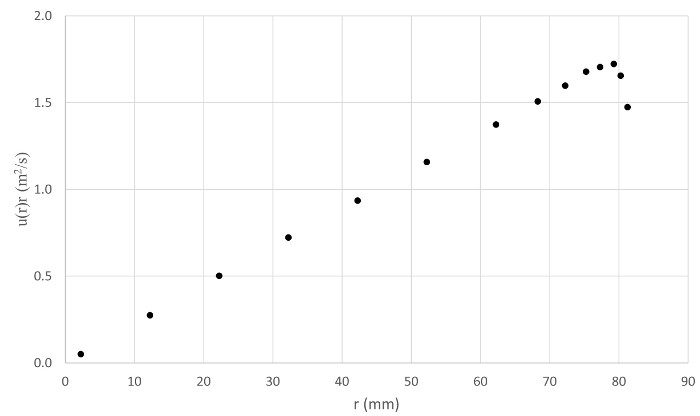
At each position, r, of the Pitot tube across the diameter of the flow passage, you have a measurement of the difference between total pressure and the static pressure. For each data point, calculate the flow velocity and enter its value in the results table. Repeat for all data points in the table, and then plot the velocity profile across the pipe. Now, calculate the discharge coefficient. To do so, first you need to plot the product between velocity and radius in function of radius. Since the velocity measurements are carried out at discrete positions, the integral in the formula for the discharge coefficient must be solved numerically using, for example, the trapezoidal rule. Next, calculate the discharge coefficient using the value of the integral together with the values recorded in the parameter table for the fluid density, the passage radius, and the measured difference between the atmospheric pressure and the static pressure at port two. Repeat these calculations for each set of data corresponding to every experimental value of the flow rate inside the passage. Now, take a look at your results.
Make a scatter plot of the discharge coefficients for different flow rates versus the values of the square root of one minus the pressure ratio. Fit a power-law function to the scatter plot, and determine a general relationship between the discharge coefficient, and the ratio between the static pressure at the flow passage and the local atmospheric pressure. Next, substitute this relationship in the equation for the flow rate. Here the density can be expressed for convenience in terms of atmospheric pressure and absolute temperature using the ideal gas law. This expression of the flow rate was, thus, developed to keep its validity under changes in local atmospheric conditions, passage size, and unit system. In summary, to calibrate a passage as a flow meter, it is necessary to establish a relationship between the flow rate and an easy-to-measure variable such as pressure difference.
The control volume method for mass conservation has a wide range of applications across the field of mechanical engineering. A Venturi tube is a device used in confined flows to determine flow rate based on pressure changes between two different sections of the passage. The method presented in this video can be used to correct for boundary layer effects inside the Venturi tube, and determine the device’s discharge coefficient. The control volume analysis for mass conservation can be used to assess flow rate for large-scale hydraulic systems by comparing the depth of flow before and after the flow restrictions.
You’ve just watched Jove’s Introduction to Control Volume Analysis for Mass Conservation. You should now understand how to apply this method to measure the flow rate across a flow passage and determine the discharge coefficient of the system. Thanks for watching.
 ) at different radial locations inside the pipe after traversing with the Pitot tube. These values were used to determine the local velocity at those radial locations, and the results are shown in Figure 3B. After using the trapezoidal rule on these data to solve equation (4) for the average velocity, we obtained a value of
 m/s. On the other hand, the value of
  from Table 1 was used to determine the ideal velocity from equation (5):
  m/s. Hence, the discharge coefficient for this flow condition is:
  . This value is shown in Figure 4 as a red triangle.
 :
: (11)
(11) :
: (12)
(12) . Consequently, equation (12) is valid for any system of units as long as the variables are consistently assigned the corresponding units. For convenience, the density from equation (7) was expressed in terms of the atmospheric pressure and absolute temperature using the ideal gas law. Equation (12) is valid for different atmospheric conditions as it accounts for changes in local pressure and temperature (T and Patm). Also, as long as geometric similarity is conserved, this equation would be valid for passages of different sizes as accounted by the radius R.
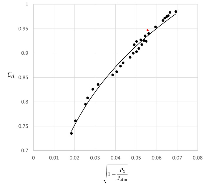
 : Discharge coefficients determined at different flow rates.
  : Discharge coefficient determined with the velocity measurements demonstrated herein. – : Power law fitted to the experimental data.