Science Education
>

Excitonic Hamiltonians for Calculating Optical Absorption Spectra and Optoelectronic Properties of Molecular Aggregates and Solids

PREPARAZIONE ISTRUTTORI
CONCETTI
Student Protocol
JoVE Journal
Chimica
È necessario avere un abbonamento a JoVE per visualizzare questo.  Accedi o inizia la tua prova gratuita.
JoVE Journal Chimica
Excitonic Hamiltonians for Calculating Optical Absorption Spectra and Optoelectronic Properties of Molecular Aggregates and Solids

1. Splitting the multi-molecular system into individual molecules

  1. Generate the structure of the system for which the excitonic Hamiltonian needs to be constructed in Tripos MOL2 molecular file format. This structure can be a snapshot from a molecular dynamics or Monte Carlo simulation of the system.
  2. If all molecules in the system consist of the same number of atoms, use the python 2.7 script getMonomers.py to generate files that contain the Cartesian coordinates for atoms in individual molecules that compose the system. Molecules that make up the system do not have to be identical (e.g., they can be isomers). This script takes two input parameters.
    1. Specify the name of the Tripos MOL2 file that contains the geometry of the system from step 1.1 (a string).
    2. Specify the number of atoms in each individual molecule that makes up the system (an integer). To complete this step, use the command:
      ./getMonomers.py YLD124-300K_0-210000.mol2 125
      Takes the structure that is contained in the sample file YLD124-300K_0-210000.mol2 on Github; writes Cartesian coordinates of individual molecules to files monomer_N.com in XYZ format, where N is a four-digit number that identifies the molecule in the system.
  3. If a system consists of molecules with different numbers of atoms, generate the structures for individual molecules using an alternative script or manually. The procedure described in subsequent steps can be used without any modifications.

2. Generating ground state point charges for atoms in individual molecules

  1. Set up a plain text file, chargeOptions.txt, with the options for a Gaussian DFT calculation of the atomic point charges in the ground state of an electrically neutral molecule. In order to obtain a reasonably accurate charge distribution for transitions with charge-transfer character, it is recommended to specify the parameters as follows.
    1. Use a long-range corrected density functional (such as ωB97X)34.
    2. Use a sufficiently large basis set that includes at least d polarization functions on non-hydrogen atoms (such as 6-31G*)35,36.
    3. Use a superfine integration grid.
    4. Use a very tight self-consistent field convergence criterion (energy convergence to 10–10 Hartree).
    5. Use atomic point charges that are fit to reproduce the electrostatic potential in the vicinity of the molecule, as is done in the CHelpG method37, because the calculated atomic charges will be used to represent the electrostatic environment.
      NOTE: In typical molecular aggregates and solids distances between molecules are relatively large, so it is often acceptable to use other atomic point charge definitions, such as Mulliken charges38.
    6. Include the NoSymm keyword in the input file to ensure that the atomic coordinates in the Gaussian output file are written in input orientation, rather than in standard orientation.
    7. Specify the name of the calculation in the comment line of the Gaussian input file.
    8. Specify the charge and multiplicity of the molecule (0 and 1, respectively) in a separate line. Sample calculation options specified in the file chargeOptions.txt may be:
      #p wB97X/6-31G* Integral(Grid=SuperFineGrid) NoSymm SCF(Conver=10) Pop=CHelpG
      Monomer charges
      0 1
  2. Set up the Gaussian input files for all individual molecules that make up the system using the parameters in the file chargeOptions.txt. This step can be efficiently accomplished using the following Bash script:
    for f in monomer_*.xyz
    do
      cat chargeOptions.txt > ${f%xyz}com
      tail -n +3 $f >> ${f%xyz}com
      echo "" >> ${f%xyz}com
    done
    NOTE: The script will produce Gaussian input files with the same names as the XYZ files generated in step 1.2, but with the extension .com. These files will contain the calculation options specified in chargeOptions.txt and the atomic coordinates from the respective .xyz files, terminated by a blank line.
  3. Run the Gaussian calculations, specifying the output file name to be the same as the input .com filename, but with the extension .log.
  4. Extract the CHelpG atomic point charges from the Gaussian output files with the extension .log, using the python 2.7 script getCHelpG.py. The script takes 2 input parameters: the name of the Gaussian output file with the extension .log and the number of atoms in a single molecule.
    NOTE: The script getCHelpG.py writes a file with the same name as the Gaussian output file, but with the extension .chg. There are 4 columns in this file: the first three with the Cartesian coordinates of atoms in the molecules, the last one with the CHelpG atomic point charges. The following Bash script can efficiently extract charges from all files:
    for f in monomer_*.log; do ./getCHelpG.py $f N; done
    (N is the number of atoms in a molecule.)
  5. If a definition of the atomic point charges other than CHelpG was used in step 2.1, extract the charges from the Gaussian output file using an alternative script or manually.

3. Calculating the excitation energies and transition densities of individual molecules in the material in the presence of an electrostatic environment

  1. Set up a plain text file, monomerOptions.txt, with the options for a Gaussian TD-DFT calculation of the excited state energies and ground-to-excited state transition density matrices for individual monomers. Suggested parameters are the same as those used for the calculation of the atomic point charges in step 2.1.
    1. Use a range-separated density functional, such as ωB97X34.
    2. Use a sufficiently large basis set that includes at least d polarization functions on non-hydrogen atoms (such as 6-31G*)35,36.
    3. Use a superfine integration grid.
    4. Use a very tight self-consistent field convergence criterion (energy convergence to 10–10 Hartree).
    5. Include the NoSymm keyword to ensure that the atomic coordinates in the Gaussian output file are written in input orientation, rather than in standard orientation;
    6. In order to obtain reasonably accurate transition densities, set a low threshold for printing eigenvector components (i.e., even coefficients for basis functions with very small contributions to an eigenvector – ideally, at least to the order of 10–5 – should be printed to the output file).
      NOTE: To set this condition, one needs to use Gaussian internal options: set overlay 9, option 40 to the absolute value of the exponent for the threshold for printing eigenvector components (e.g., IOp(9/40) = 5 sets the cutoff threshold to 10–5).
    7. Specify the name of the calculation in the comment line of the Gaussian input file.
    8. Specify the charge and multiplicity of the molecule (0 and 1, respectively) in a separate line. Sample calculation options specified in the file monomerOptions.txt may be:
      #p tda(NStates=10) wB97X/6-31G* Integral(Grid=SuperFineGrid) NoSymm SCF(Conver=10) iop(9/40=5)
      Monomer with charges
      0 1
  2. Set up the Gaussian input files for the calculation of the excitation energies and transition densities of all individual molecules in the material in the presence of an electrostatic environment represented by the point charges on all other molecules in the material, with file name monomer_N_wCh.com.
    1. Include a request to save a Gaussian checkpoint file with filename monomer_N_wCh.chk in the Gaussian input file.
      NOTE: For the naming convention described in this protocol, this step can be accomplished using the python 2.7 script getMonomerWCh.py that reads in the calculation options specified in the file monomerOptions.txt, the atomic coordinates for individual molecules in the system that are stored in files monomer_N.xyz, and atomic point charges for all individual molecules that are stored in files monomer_N.chg (N is the number of the monomer).
  3. Run the Gaussian calculations, specifying the output file name to be the same as the input .com filename, but with the extension .log. The calculation will also save a checkpoint file with the same filename, but with the extension .chk.

4. Extracting excitation energies for bright states of individual molecules that make up the system from the Gaussian output files

  1. Copy the excitation energies for the bright excited states of individual monomers from the Gaussian output files with the extension .log to a plain text file called all_energies.txt.
    NOTE: If there is only one bright excited state and all Gaussian output files are in the same directory, then this step can be efficiently accomplished by creating an empty plain text file, all_energies.txt, then appending the line in the output file that contains the excitation energy of the bright state for each monomer using the following Bash script:
    for f in monomer*WCh.log; do grep "Excited State M" $f >> all_energies.txt; done
    (M is the number of the excited bright state; the number of spaces between the word State and the number M should be the same as in the Gaussian output files.)
  2. In the file all_energies.txt, keep only the column that contains the numerical values of the excitation energies (in eV); delete all other columns.

5. Calculating the excitonic couplings for all pairs of molecules that make up the molecular system

  1. Convert the checkpoint files to human-readable format using the formchk utility that is part of Gaussian using the following Bash script:
    for f in monomer_*.chk; do formchk $f; done
    NOTE: The human-readable formatted checkpoint files will have the same name as the original checkpoint files, but with the extension .fchk.
  2. Use the python 2.7 script switchSign.py that takes the name of the Gaussian output file with the extension .log and the number of excited states N included in the calculation as input parameters.
    NOTE: This script prints out the contents of the .log file switching the direction of the transition dipole moment vectors from the ground to all excited states if the angle between the ground state permanent dipole moment vector and the transition dipole moment vector for the ground to first excited state transition is obtuse.
  3. Save the output produced by the script switchSign.py to a file that has the same name as the .log file, but with the extension .log2.
  4. For molecules where the angle between the ground state permanent dipole moment vector and the transition dipole moment vector for the ground to first excited state transition is acute, copy the .log file to a file with the same name and extension .log2.
    NOTE: If the naming convention recommended in this protocol is used, steps 5.2–5.4 can be accomplished efficiently for all individual monomers using the following Bash script:
    for f in monomer*_wCh.log
    do
      ./switchSign.py $f 10 > ${f}2
      if [ -s ${f}2 ]
      then
        echo 'Switching transition dipole moment signs for' $f
      else
        echo 'Copying' $f 'to' ${f}2
        cp ${f} ${f}2
      fi
    done
  5. Use the Multiwfn multifunctional wavefunction analyzer to write the transition density cube file based on the Gaussian formatted checkpoint file with the extension .fchk and the processed Gaussian output file with the extension .log2.
    NOTE: Gaussian only natively supports saving the spatial density distribution to a density cube file for observables that correspond to Hermitian operators. Because the transition density operator is not Hermitian, a postprocessing program is required to obtain a density cube file.
    1. Launch the Multiwfn program.
    2. Submit the Gaussian formatted checkpoint file (the file with the extension .fchk generated in step 5.1) as the input file.
    3. Select option 18, Electron excitation analysis, from the Main function menu.
    4. Select option 1, Analyze and visualize hole-electron distribution, transition dipole moment and transition density, from the Electron excitation analyses menu.
    5. Submit the Gaussian output file with adjusted signs for the transition dipole vectors (the file with the extension .log2 saved in step 5.2) when prompted to Input the path of the Gaussian output file or plain text file containing excitation data.
    6. Specify the transition for which the transition density cube file should be generated (if there is only one bright state, it is the transition from the ground state to that state).
    7. Select option 1, Visualize and analyze hole, electron and transition density and so on, in the next menu.
    8. Select the number of points in the grid for which the transition density cube file will be generated: a larger number of points results in more accurate excitonic couplings, but increases the calculation time significantly, in most cases, option 1, Low quality grid, covering whole system, about 125000 points in total, is sufficient.
    9. Select option 13, Output cube file of transition density to current folder, in the following menu. Transition density cube file transdens.cub will be written, rename this file to have the same name as the .log2 and .fchk files, with the extension .cub.
      NOTE: Multiwfn is intended to run interactively, with calculation options entered from the keyboard in response to prompts. However, it is more convenient to set up a file with processing options and then to have Multiwfn read them from that file.
  6. To efficiently generate set up files with Multiwfn processing options for all .fchk files in the current directory, use the Bash script makeOpt.sh. The files written by the script makeOpt.sh have the same names as the .fchk files with the extension .opt.
  7. Generate the transition density cube files in a single batch using the following Bash script:
    for f in monomer*_wCh.fchk
    do
      Multiwfn $f < ${f%fchk}opt
      mv transdens.cub ${f%fchk}cub
    done
    NOTE: Figure 1 shows the transition density for a molecule of 2-[4-[(E,3E)-3-[3-[(E)-2-[4-[bis[2-[tert-butyl-(dimethyl)silyl]oxyethyl]amino]phenyl]ethenyl]-5,5-dimethylcyclohex-2-en-1-ylidene]prop-1-enyl]-3-cyano-5-phenyl-5-(trifluoromethyl)furan-2-ylidene]propanedinitrile (commonly referred to as YLD 124 [Jen2005])39 in the presence of point charges of surrounding molecules.
  8. Convert .cub files to files that explicitly specify the coordinates of the centers of all cubes on the grid used in step 5.5.8 (first 3 columns) and the values of the transition density inside the cube (last column) using the python 2.7 script cubeFormat.py. The script takes the name of a .cub file as input. To convert all .cub files in a directory, use the Bash script:
    for f in monomer_0*.cub; do echo $f; ./cubeFormat.py $f; done
    NOTE: The script cubeFormat.py writes a formatted density cube file with the same name as the input file it takes, but with the extension .fcub.
  9. Use the .fcub files generated in step 5.8 to calculate the excitonic couplings between all pairs of molecules in the system using the transition density cube method31. This step can be accomplished using the cubePairGen program that takes two .fcub files for different molecules as input. To run it, use the command:
    ./cubePairGen monomer_N_wCh.fcub monomer_M_wCh.fcub
    NOTE: The program returns a file named coup_N_M with a single line that contains three numbers: the molecule numbers N and M, followed by the excitonic coupling between these two molecules in eV. The program source code in the file CubePairGen.cpp can be compiled using the C++ compiler in the GNU Compiler Collection with the command:
    g++ CubePairGen.cpp –o cubePairGen
  10. If the file naming convention suggested in this protocol is used, the calculations can be run as a batch for all pairs of individual molecules that make up the system studied. To run these calculations, use the following Bash script:
    for f in *.fcub
    do
      for g in *.fcub
      do
        ff=${f#monomer_}
        gg=${g#monomer_}
        fff=${ff%_wCh*}
        ggg=${gg%_wCh*}
        if [ "$fff" -gt "$ggg" ]
        then
    (*) ./cubePairgen' $f $g '> coup_'${fff}'_'${ggg}
        fi
      done
    done
    NOTE: Figure 2 shows the transition densities for two molecules of YLD 124 that are used to calculate the excitonic coupling between these molecules. For large systems, where the total number of molecule pairs is large, the line marked by an asterisk in the Bash script can be modified to submit calculations to a supercomputing cluster’s queuing system.
  11. Once the calculations in step 5.8 are finished, create an empty file all_couplings.txt and combine all excitonic couplings into a single file using the following Bash script:
    for f in coup_0*; do cat $f >> all_couplings.txt; done

6. Setting up the excitonic Hamiltonian

  1. Combine the excited state energies in the file all_energies.txt that was generated in step 4.2 and the excitonic couplings in the file all_couplings.txt that was generated in step 5.9 into a single file that contains the complete excitonic Hamiltonian matrix using the python 2.7 script SetupHam.py using the terminal command:
    ./Setup_Ham.py all_energies.txt all_couplings.txt N >Hamiltonian.txt
    NOTE: The program will write a file Hamiltonian.txt with three columns: the row number, column number, and value in eV for each matrix element, with rows separated by blank lines.
    1. Specify the name of the file that contains excitonic energies.
    2. Specify the name of the file that contains excitonic couplings.
    3. Specify the dimension N of the Hamiltonian matrix (the number of molecules in the system).

Excitonic Hamiltonians for Calculating Optical Absorption Spectra and Optoelectronic Properties of Molecular Aggregates and Solids

Learning Objectives

In this section we present representative results for computing the optical absorption spectrum of an aggregate of six YLD 124 molecules, shown in Figure 3a, where the structure of the aggregate was obtained from a coarse-grained Monte Carlo simulation. YLD 124 is a prototypical charge-transfer chromophore that consists of an electron-donating group of diethyl amine with tert-butyldimethylsilyl protecting groups that is connected via a π -conjugated bridge to the electron accepting group 2-(3-cyano-4,5,5-trimethyl-5H-furan-2-ylidene)-malononitrile39. This molecule has a large ground-state dipole moment, ~30 D. Electronic structure calculations for individual molecules were performed using the ωB97X34 functional with the 6-31G* basis set35,36. TD-DFT calculations used the Tamm-Dancoff approximation40. Partial atomic charges were computed with the CHelpG population analysis method37.

The Hamiltonian for this system, constructed using the protocol described in this paper, is shown in Table 1.

The absorption spectrum calculated for this excitonic Hamiltonian is shown in blue in Figure 3b. Because there are six molecules with only a single bright excited state for each molecule, a 6-by-6 excitonic Hamiltonian was generated, resulting in six transitions. The eigenvalues of this Hamiltonian are the lowest six excited state energies for the molecular aggregate. The height of the vertical lines represents the oscillator strength fi for each transition from the ground to the ith excited state of the molecular aggregate. It can be found using the expression29

Equation 2

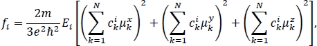
where m is the electron mass, e is the elementary charge, ħ is the reduced Planck’s constant, N is the total number of molecules in the aggregate, Ei is the eigenvalue that corresponds to the ith excited state of the molecular aggregate, cki is the expansion coefficient for the contribution of the kth molecule in the aggregate to the ith excited state of the aggregate written in the basis of bright excited states on individual molecules, and μkα are the components of the transition dipole moment vector for the ground to bright excited state of the kth molecule in the aggregate, α = x, y, z . The values of Ei and cki are found by solving the eigenvalue equation for the Hamiltonian matrix (the time-independent Schrödinger equation). The values of μkα can be found in the “.log2” files that are generated in step 5.2 of the protocol. The total spectrum is a smooth line created by summing over Gaussian functions centered at each of the excitation energies and weighted by the corresponding oscillator strengths29.

For comparison, the spectrum computed from an all-electron TD-DFT calculation on the entire molecular aggregate is shown in magenta. For these spectra, the integrated intensity of the exciton spectrum is larger than the TD-DFT spectrum (Iexc/ITD-DFT = 1.124) and the difference in the mean absorption energies is Eexc – ETD-DFT = 0.094 eV. These offsets are systematic for molecular aggregates of a given size and can be corrected for to obtain very good agreement between exciton model and TD-DFT spectra. For instance, for a set of 25 molecular aggregates that each consists of 6 YLD 124 molecules, the average integrated intensity ratio Iexc/ITD-DFT = 1.126, with a standard deviation of 0.048, and the difference in the mean absorption energies is Eexc – ETD-DFT = 0.057 eV, with a standard deviation of 0.017 eV. The exciton model and TD-DFT spectra shown in Figure 3b also have similar shapes, as characterized by Pearson’s product-moment correlation coefficient41 between them of 0.9818 and Pearson’s product-moment correlation coefficient between their derivatives of 0.9315. On average, for a set of 25 molecular aggregates that each consists of 6 YLD 124 molecules, the agreement in spectral shape is even better than for the example shown, with values of 0.9919 (standard deviation of 0.0090) and 0.9577 (standard deviation of 0.0448) for the two Pearson’s coefficients, respectively29. Our earlier work suggests that the spectral shape is primarily determined by local electrostatic interactions between chromophores in the aggregate that are accounted for in the exciton model described in this paper, whereas the excitation energy and intensity depend considerably on the mutual polarization between the chromophore and its environment that the model neglects29.

Figure 1
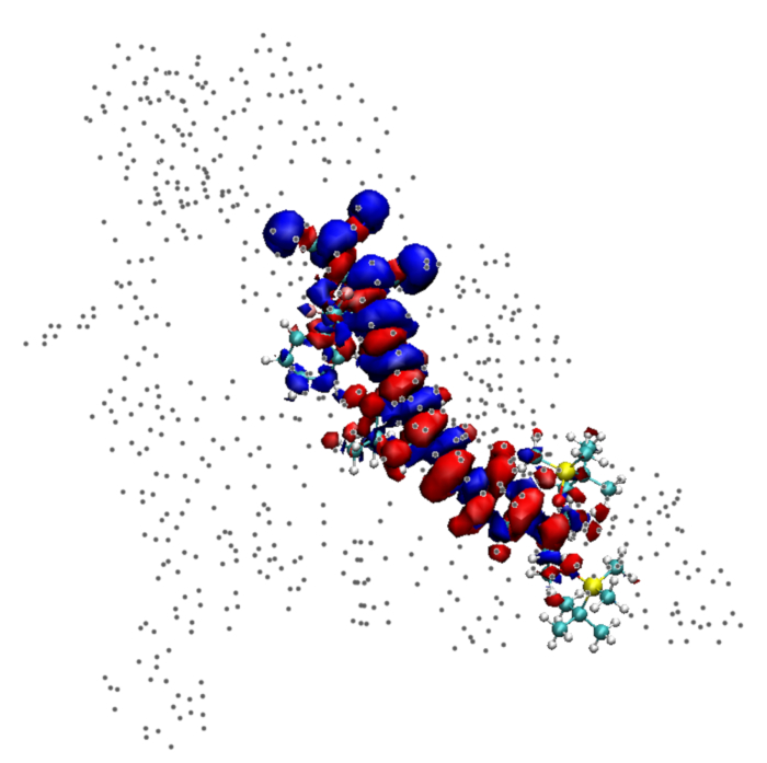
Figure 1: An isosurface for the transition density plotted for a single molecule of YLD 124. The the positions of atomic charges on surrounding molecules are shown by gray dots. Please click here to view a larger version of this figure.

Figure 2
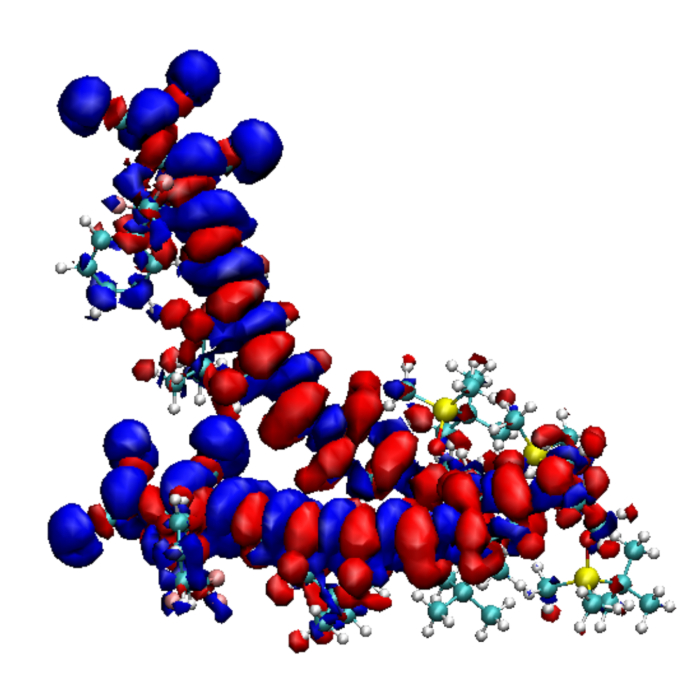
Figure 2: The transition densities plotted for two molecules of YLD 124, i and j, that are used for computing the excitonic coupling bij between these molecules. The surrounding charges are not shown. Please click here to view a larger version of this figure.

Figure 3
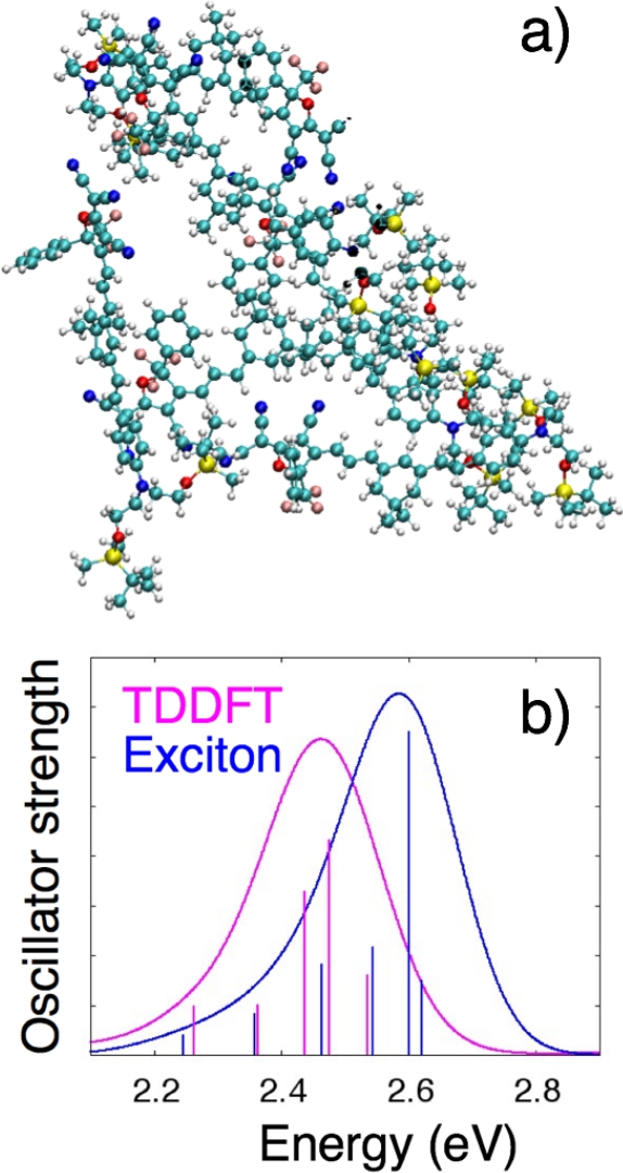
Figure 3: The structure and calculated spectrum for an aggregate of six YLD 124 molecules. (a) The aggregate structure used in the sample calculation. (b) The corresponding absorption spectra created using the exciton model Hamiltonian (blue) and an all-electron TD-DFT calculation on the entire aggregate (magenta). Please click here to view a larger version of this figure.

2.4458 -0.0379 -0.0899 0.0278 -0.0251 0.0120
-0.0379 2.4352 -0.0056 -0.1688 -0.0070 -0.0085
-0.0899 -0.0056 2.5111 0.0032 0.0239 0.0794
0.0278 -0.1688 0.0032 2.3954 0.0057 0.0073
-0.0251 -0.0070 0.0239 0.0057 2.5171 -0.0211
0.0120 -0.0085 0.0794 0.0073 -0.0211 2.5256

Table 1: The Hamiltonian for a sample calculation on the aggregate of six YLD 124 molecules shown in Figure 3a. The diagonal elements are the excitation energies of individual molecules; the off-diagonal elements are the excitonic couplings between molecules (all values are in eV).

List of Materials

Gaussian 16, revision B1
Multiwfn version 3.3.8
GNU compiler collection version 9.2
python 2.7.0

Lab Prep

Rational design of disordered molecular aggregates and solids for optoelectronic applications relies on our ability to predict the properties of such materials using theoretical and computational methods. However, large molecular systems where disorder is too significant to be considered in the perturbative limit cannot be described using either first principles quantum chemistry or band theory. Multiscale modeling is a promising approach to understanding and optimizing the optoelectronic properties of such systems. It uses first-principles quantum chemical methods to calculate the properties of individual molecules, then constructs model Hamiltonians of molecular aggregates or bulk materials based on these calculations. In this paper, we present a protocol for constructing a tight-binding Hamiltonian that represents the excited states of a molecular material in the basis of Frenckel excitons: electron-hole pairs that are localized on individual molecules that make up the material. The Hamiltonian parametrization proposed here accounts for excitonic couplings between molecules, as well as for electrostatic polarization of the electron density on a molecule by the charge distribution on surrounding molecules. Such model Hamiltonians can be used to calculate optical absorption spectra and other optoelectronic properties of molecular aggregates and solids.

Rational design of disordered molecular aggregates and solids for optoelectronic applications relies on our ability to predict the properties of such materials using theoretical and computational methods. However, large molecular systems where disorder is too significant to be considered in the perturbative limit cannot be described using either first principles quantum chemistry or band theory. Multiscale modeling is a promising approach to understanding and optimizing the optoelectronic properties of such systems. It uses first-principles quantum chemical methods to calculate the properties of individual molecules, then constructs model Hamiltonians of molecular aggregates or bulk materials based on these calculations. In this paper, we present a protocol for constructing a tight-binding Hamiltonian that represents the excited states of a molecular material in the basis of Frenckel excitons: electron-hole pairs that are localized on individual molecules that make up the material. The Hamiltonian parametrization proposed here accounts for excitonic couplings between molecules, as well as for electrostatic polarization of the electron density on a molecule by the charge distribution on surrounding molecules. Such model Hamiltonians can be used to calculate optical absorption spectra and other optoelectronic properties of molecular aggregates and solids.

Procedura

Rational design of disordered molecular aggregates and solids for optoelectronic applications relies on our ability to predict the properties of such materials using theoretical and computational methods. However, large molecular systems where disorder is too significant to be considered in the perturbative limit cannot be described using either first principles quantum chemistry or band theory. Multiscale modeling is a promising approach to understanding and optimizing the optoelectronic properties of such systems. It uses first-principles quantum chemical methods to calculate the properties of individual molecules, then constructs model Hamiltonians of molecular aggregates or bulk materials based on these calculations. In this paper, we present a protocol for constructing a tight-binding Hamiltonian that represents the excited states of a molecular material in the basis of Frenckel excitons: electron-hole pairs that are localized on individual molecules that make up the material. The Hamiltonian parametrization proposed here accounts for excitonic couplings between molecules, as well as for electrostatic polarization of the electron density on a molecule by the charge distribution on surrounding molecules. Such model Hamiltonians can be used to calculate optical absorption spectra and other optoelectronic properties of molecular aggregates and solids.

Tags