These results provide the steps for the construction of a 3D mesh that simulates a dendritic spine with a spine head and spine neck (Figure 1 a Figure 4). In addition, multiple dendritic spines can be inserted in a single dendritic segment (Figure 5) to study heterosynaptic plasticity of AMPARs14. The PSD on the top of the spine head (Figure 6) is the place where synaptic anchors bind to AMPARs and trap them temporarily at the synapse (Figure 7, Figure 8).
Synaptic plasticity could be verified roughly through changes in the number of species of anchor_AMPAR, anchor_AMPAR_LTP, and anchor_AMPAR_LTD at each spine. For the exact calculation of the occurrence of synaptic plasticity, it is recommended to calculate the variation in the total number of anchored and free AMPARs at the synapse. This can be performed using third-party programs to open the saved data of the simulation to summate the time series of the free AMPARs and the anchored AMPARs at each PSD (Figure 8).
The release of AMPARs on the mesh allowed the observation of their diffusion by a stochastic random walk along the dendrite and dendritic spines. Factors that modify the affinity of AMPARs for the anchors, such as posttranslational modifications and alterations of the rates of endocytosis and exocytosis, can trap the AMPARs at the PSD24,25,26. The binding of AMPARs with the anchors located at the PSD trapped a high density of AMPARs at the synapse. Homosynaptic potentiation (Figure 9) and depression (Figure 10) could be verified respectively through increases and decreases in the number of anchored AMPARs caused by changes in the affinity of AMPARs by anchors in comparison to the basal condition (Figure 11). Factors that reduced the affinity of AMPARs with the anchors released multiple AMPARs from one dendritic spine (i.e., homosynaptic depression) and induced heterosynaptic potentiation at the neighboring spines. Also, factors that increased the affinity of AMPARs for the anchors at one spine induced homosynaptic potentiation at that spine and heterosynaptic depression at the neighboring spines14. In this way, heterosynaptic plasticity was observed as the opposite effect at the neighboring spines of the homosynaptic plasticity induced at a given spine. For instance, homosynaptic LTP induction at a single spine created a heterosynaptic LTD effect at the neighboring spines (Figure 8E,F,G).
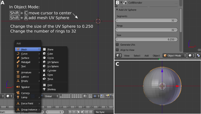
Figure 1: Creation of the dendritic spine head using a spherical mesh. (A) Adding the UV sphere. (B) Setting up the sphere dimensions. (C) Observing the created sphere. Please click here to view a larger version of this figure.
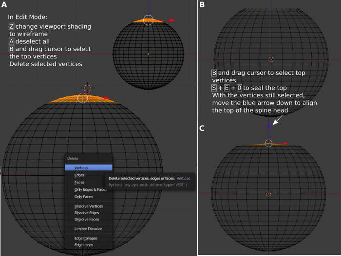
Figure 2: Construction of the top region. (A) Selecting the top region of the sphere. (B) Removing the selected region to make it flat. (C) Sealing the flat top. Please click here to view a larger version of this figure.
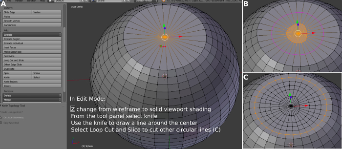
Figure 3: Creating concentric areas on the top of the spine. (A) Visualizing the top. (B) Using a knife to define a concentric region. (C) Creating multiple concentric regions. Please click here to view a larger version of this figure.
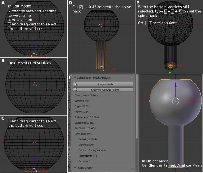
Figure 4: Creating the dendritic spine neck. (A) Selecting the bottom of the modified sphere. (B) Deleting the selected vertices. (C) Selecting the bottom. (D) Extrusion of the bottom to create the spine neck. (E) Sealing the bottom of the spine neck. (F) Analyzing the created spine. Please click here to view a larger version of this figure.
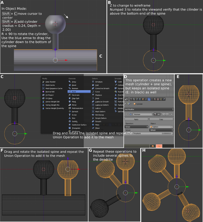
Figure 5: Creation of the dendrite with multiple spines. (A) Using the cylindrical mesh to create a dendrite. (B) Aligning the dendritic spine with the cylinder. (C) Joining the cylinder with the spine. (D) The Boolean operation to join the meshes. (E) The new combined mesh. (F) Adding the second spine. (G) Adding the third spine. (H) Adding the fourth spine. Please click here to view a larger version of this figure.
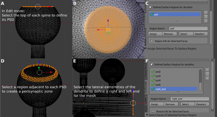
Figure 6: Defining the PSD region and the perisynaptic zone. (A) Selecting the PSD region. (B) Detailed view of the created PSD. (C) Defining the PSD surface region. (D) Selecting and defining the perisynaptic zone around the PSD. (E) Selecting and defining the lateral surface of the dendrite. (F) Defined surface regions. Please click here to view a larger version of this figure.
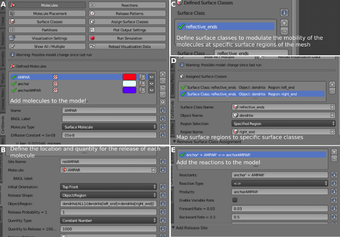
Figure 7: Defining the surface molecules. (A) Defining AMPAR, anchor, and AMPAR bound to anchor. (B) Defining the location and quantity of AMPAR copies. (C) Defining the Surface Classes. (D) Assigning the Surface Classes. (E) Creating the chemical reactions between the molecules. Please click here to view a larger version of this figure.
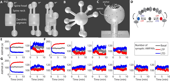
Figure 8: Representative results of synaptic plasticity. (A) Different meshes of a dendritic segment with two, four, or eight spines. (B) A different view of the dendritic segment with eight spines. (C) Detailed view of a dendritic spine with AMPARs and anchors at the PSD. (D) Diagram of the trafficking of AMPARs in and out of the PSD through their interactions with the anchors. (E-G) The curves show the number of synaptic AMPARs at each PSD for the basal condition and during LTP and LTD. The induction of homosynaptic LTP or LTD at a single spine created a heterosynaptic effect in the nearby spines for the mesh with two spines (E), four spines (F), and eight spines (G). Please click here to view a larger version of this figure.
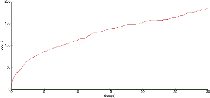
Figure 9: Representative result of the LTP condition. (A) The x-axis is the time and the y-axis is the number of the complex anchor_LTP_AMPAR at PSD1. There was a release of 200 free anchor_LTP at the beginning of the simulation. A higher number of bonds with anchors was formed in comparison to the basal condition (Figure 11) Please click here to view a larger version of this figure.
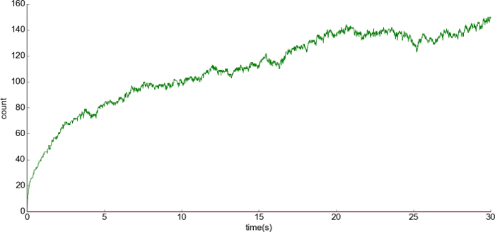
Figure 10: Representative result of the LTD condition. (A) The x-axis is the time and the y-axis is the number of the complex anchor_LTD_AMPAR at PSD1. There was a release of 200 free anchor_LTD at the beginning of the simulation. A lower number of bonds with anchors was formed in comparison to the basal condition (Figure 11). Please click here to view a larger version of this figure.
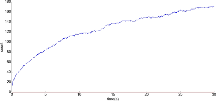
Figure 11: Representative result during basal condition. (A) The x-axis is the time and the y-axis is the number of the complex anchor_AMPAR at PSD1. There was a release of 200 free anchors at the beginning of the simulation. Please click here to view a larger version of this figure.
Supplementary File 1. Please click here to download this file.