Science Education
>

A Machine-Vision Approach to Transmission Electron Microscopy Workflows, Results Analysis and Data Management

PREPARAZIONE ISTRUTTORI
CONCETTI
Student Protocol
JoVE Journal
Biologia
This content is Free Access.
JoVE Journal Biologia
A Machine-Vision Approach to Transmission Electron Microscopy Workflows, Results Analysis and Data Management

1. Method 1: Dose calibration of the transmission electron microscope for TEM and scanning TEM (STEM) imaging modes

  1. Turn on the picoammeter and allow it to warm up for a minimum of 30 min before starting a dose calibration. Load the dose calibration holder into the TEM and connect the calibration holder to the picoammeter using the quick-connect cable.
  2. With the microscope in TEM mode, open the column valves and locate the 35 µm fiducial hole on the dose holder (Figure 2). Launch the MVS software application and select Dose (Calibration Automation) from the experiment options.
    NOTE: The fiducial hole location is saved by the software after the initial calibration, enabling the software to automatically locate its position for future calibrations.
  3. Click on the Connect icon (Figure 1A) and select the microscope to activate the connection between the TEM and the MVS software. Once connected, the images from the camera/detector will be visible in the image viewer of the software.
    NOTE: It is not necessary to optimize the eucentric height, and the edge of the fiducial hole may appear blurry due to the thickness of the tip. This will not affect the current measurements.
  4. Navigate to the Dose tab and then to Dose Calibration. Select Dose Area Calibration process, follow the software prompts, and enter the requested user-configurable values (such as the aperture and monochromator settings). After the Dose Area Calibration is complete, select the Dose Current Calibration process and follow the software prompts.
  5. Repeat the calibration process (step 1.4) for each spot size, aperture, or monochromator setting that may be utilized during the experiment.
  6. When the calibration process for TEM mode is finished, calibrate the electron dose for STEM mode by repeating step 1.4.
    NOTE: STEM mode does not require the Dose Area Calibration to be performed.
  7. When all desired calibrations are finished, click on Close Session, remove the dose calibration holder, and return to the start screen of the MVS software.

2. Method 2: Determination of dose threshold using the MVS and dose software

  1. Load a standard TEM grid with a sample (commercially available ZSM-5 zeolite nanoparticles were used in this example) into a standard TEM holder. Insert the holder into the TEM and locate a region of interest (crystalline zeolite nanoparticles).
  2. Open the MVS software application and select Altro.
    NOTE: Additional information about the sample (e.g. sample identifier and description, the operator name, and experiment notes) can be added to the experimental parameters field.
  3. Repeat step 1.3 to connect to the MVS software and navigate to the image metadata tab in the MVS software interface to select the following metadata to overlay on the image stream shown in the live display: Magnification, Max Dose, and Dose Rate. Other metadata may be included if the user desires. A screenshot of the MVS software interface showing the dose management controls is provided in Supplementary File 1.
  4. Open the Dose tab and select Dose Management and Enable Dose Monitoring to activate automated electron dose tracking. Select Show Dose Layer to display the dose color overlay.
  5. Set the values for the high dose level and the high dose rate and press on Save (in this example, values of 60,000 e2 and 500 e2·s, respectively, were used).
  6. Navigate to the Settings tab, select Dose, and set the Dose Navigation Map Opacity and Dose Image Overlay Opacity values (in this example, values of 0.50 and 0.30, respectively, were used).
  7. In the Live Image Viewer window, activate drift correction by clicking on Drift Correct.
  8. Navigate to the Data View tab and plot the metadata values Defocus and Focus Quotient on the Y axis.
    NOTE: Any of the available metadata values can be plotted in real time during the experiment from the data view table.
  9. Activate Focus Assist, and then select Calibrate Focus to run the automated focus assist calibration. Once the Calibrate Focus routine is complete, close the Data View tab.
  10. Open the Image Analysis tab in the MVS software and activate the Live FFT and Quadrants 1 & 2 options.
  11. Using the microscope's software controls, adjust the beam conditions so that the electron flux is ~500 e2·s. and move to a new region in the sample and center the sample ROI in the live view of the MVS software.
    NOTE: When making large stage movements, drift control and focus assist will automatically de-activate, and must be re-engaged once the new ROI is selected.
  12. Make a note of the dose conditions in the software using the Tag function. Highlight the Tag icon and enter the desired text to denote a specific series of images within the timeline. Images will be tagged with this text until the Tag icon is deselected.
  13. Maintain a constant dose rate while continuously imaging the same ROI until the peaks corresponding to the atomic structure in the FFT plot have disappeared.
  14. Reduce the magnification, open the Dose Management tab, and activate Show Dose Layer to overlay a color-coded dose map.
    NOTE: This feature provides a visual reference of the areas of the sample that have been exposed to the electron beam and their relative dose exposure. Highlighting these areas in individual images with the cursor will indicate their respective dose values.
  15. Disconnect and end the session by deselecting Connect, then select Close Session. Save a copy of the session data to an external source to prevent the data saved in the MVS software from being overwritten during subsequent experiments (Supplementary File 2).

3. Method 3: Metadata and trend analysis and data export using the analysis software

  1. Launch the analysis software (the offline software for viewing the fully synchronized datasets) and open the experiment session file by selecting it from the file library.
    NOTE: Users can also access the analysis software through the Review Session icon in the MVS software during an experiment.
  2. Display the drift corrected images by activating the DC tab below the Image View Port and select the desired data overlays by checking their respective Overlay Data boxes in the Image Metadata tab (in this example Microscope, Date/Time, Dose Rate, Max Dose, and Magnification were used). Other metadata may be plotted as the user desires.
  3. Check the Timeline box for Max Dose and Dose Rate to add a graphical plot of these values to the timeline. Highlight or scroll through these graphical plots to update the image displayed in the viewport. Access a variety of tools through the Notes, Image Analysis, Toolbox, and Data View tabs.
    1. Access the FFT for each image through the Image Analysis tab and click on Live FFT to update the FFT while scrolling through images.
    2. Use the fading of the FFT peaks to determine the time point at which the zeolite structure loses crystallinity. Record the max dose value recorded with that image.
  4. Use the Filter option to filter large datasets easily into smaller, sharable datasets without losing their associated metadata. Open the filter panel and adjust the sliders so that only data with a dose rate equal to or above ~500 e2·s is selected, and save the new collection using the name Dose Threshold Study.
    NOTE: Filters may be applied for any of the associated metadata types.
  5. Export the images and metadata from the session into other file types enriched with scale bars and metadata overlays.
    1. Highlight the collection in the library pane and select Publish by right-clicking the selection. From the Publish window, select the desired options for the file type export.
    2. Select the drift corrected data tab and apply overlays of any desired metadata and the FFT (position the FFT overlay as desired; examples of images exported with the FFT are shown in Figure 3).
  6. Export the image series as a movie file using the same Publish option. Select the images by highlighting them in the timeline, using the filter options or exporting the full database file. Select the desired movie format, frame rate, and file location. A movie of the zeolite degradation experiment obtained using a 200 kV TEM is provided in Supplementary File 3.
  7. Export the metadata separately from the acquired images as a CSV file by selecting the Metadata (CSV) option while publishing.
    ​NOTE: Raw and drift corrected images are exported as separate CSVs (Supplementary File 4 and Supplementary File 5).

4. Method 4: In situ heating study of gold on iron oxide nanoparticles

  1. Dropcast a nanocatalyst (Au/FeOx) suspended in ethanol onto an in situ heater E-chip, a mico-electrochmechanical (MEM) sample support, and allow it to air-dry. Mount the sample in the in situ heating holder, insert the holder with the sample into the TEM, and connect the holder to the power supply using the supplied cable. Locate a sample ROI using the TEM controls.
    NOTE: This experiment used a heating holder which is fully integrated with the MVS software, enabling temperature metadata to be embedded with the images.
  2. Select the appropriate workflow option from the MVS software (in this example, the Fusion Workflow was used, but other manufacturer heating holders can be used by selecting Altro).
  3. Follow the workflow prompts to confirm the electrical connection between the holder and the heating E-chip by loading the calibration file and performing a device check.
  4. Connect the microscope to the MVS software, as shown earlier in steps 2.3-2.10 (in this example, the metadata values for dose rate, max dose, match correlation, drift rate, and channel A temperature were selected), and center the sample ROI in the field of view.
  5. Open the Fusion AX tab and set up and apply a temperature.
  6. Click the Channel A Setup button to access the temperature control settings. Select the Temperature function and Manual control mode.
  7. Click the Experiment button to access the experimental controls. Set the Ramp Rate to 10 °C/s and the Target to 600 °C. Click on Apply to start the experiment.
    NOTE: The experiment can be paused or stopped at any time using the quick access buttons in the bottom right corner of the MVS software, without opening the Fusion AX tab.
  8. After the set temperature of 600 °C is reached, open the Fusion AX tab and select Experiment. Change the Ramp Rate to 2 °C and the Target to 800 °C. Click on Apply to start the experiment.
    NOTE: The procedure for applying a heating ramp is dependent on the in situ heating system that is used. The steps highlighted above to apply the temperature ramp apply to the system used in this example.
  9. Highlight any events or points of interest during the experiment using the tagging feature, as shown in step 2.10. Continue to image the sample and adjust the temperature profile as desired. When finished, click on End Session and save the data file using the analysis software (a portion of the database file discussed in the representative results is supplied as Supplementary File 6).
  10. Open the analysis software to review the session. Plot the temperature, template morphing factor, dose rate, and cumulative dose in the timeline. Export images and movies as desired using the steps outlined in step 3.6 and 3.7. Images and movies may be exported with or without the dose map overlays (Figure 4).

A Machine-Vision Approach to Transmission Electron Microscopy Workflows, Results Analysis and Data Management

Learning Objectives

This work highlights the utility of data acquisition using MVS software for TEM imaging and in situ experiments. Microscope alignment and condition setup were performed and selected through the TEM manufacturer's default controls. After initial setup, the protocols presented in this video article were conducted through the MVS software. A 300 kV TEM was used for all experiments presented in the video protocol and representative data, except for the comparison zeolite data which was acquired using a 200 kV cold FEG (Figure 3DF and Table 1). All metadata was collected and aligned to its respective images automatically by the MVS software.

After launching the software and selecting the appropriate workflow from the menu, a connection to the microscope is established by activating the Connect button in the toolbar in the far left of the image viewer, as shown in Figure 1A. When the Connect button is highlighted, images and associated metadata from the microscope are automatically streamed into the MVS software and appear in the image view pane. These images and their associated metadata are saved chronologically in a timeline that can be opened, reviewed, and analyzed without interrupting the recording of new data into the timeline (Figure 1B). Streaming can be interrupted by the user at any time by deactivating the Connect icon.

Once the connection is activated, other workflows that are dependent on the MVS software framework can be accessed. In the examples shown in this video protocol, a dose calibration must be performed before utilizing the other functions of the MVS software. Dose calibration is an automated process controlled by the MVS software; it uses a dedicated Faraday cup dose calibration holder to measure the beam's current and area for the combination of parameters. The Faraday cup calibration holder, shown in Figure 2, connects to an external picoammeter, which precisely measures the beam current. Once inserted in the microscope, the fiducial alignment hole is centered and the desired beam conditions to be calibrated (spot sizes, apertures, and magnifications) are entered in the software. The software performs a series of calibration steps for each combination of the selected conditions. During dose calibration, the holder automatically moves between the integrated Faraday current collector cup and the through-hole. The current measurement for each combination of lens conditions is measured on the Faraday cup by the picoammeter. Then, the software translates the stage to center the beam in the through-hole and the beam area is determined through machine-vision algorithms. This series of measurements builds a profile of the the relationship between the intensity/brightness and the beam area. This enables the software to extrapolate the beam area as the intensity/brightness setting is adjusted during an experiment regardless of the field of view. Values for cumulative dose and dose rate are calculated using these beam current and beam area measurements and a dose calibration file is generated. This process essentially defines a dose "fingerprint" for the TEM and its individual lens conditions. Once the dose is calibrated for the TEM, the user is able to operate normally and freely adjust the magnification and intensity with no loss of dose information or manual note taking17. After calibration is complete, the dose calibration holder is removed, allowing the sample to be inserted as normal. The calibration process for both the TEM and STEM modes normally takes less than 10 min.

After calibrating the dose conditions, a commercially purchased zeolite nanoparticle (ZSM-5) sample was imaged under high dose rate conditions to determine the threshold (cumulative) dose at which the sample is too damaged to provide structural information. The ZSM-5 nanoparticles were suspended in ethanol and dropcast on a conventional copper TEM grid. They were imaged continuously at 300 kV in TEM mode using a spot size of 3 and a 100 µm condenser aperture. The dose rate read by the MVS software under high dose rate conditions was 519 e2·s. Nanoparticles in the field of view were imaged continously until the peaks in the FFT disappeared, indicating degradation of the crystalline structure, as shown in Figure 3AC and Supplementary File 3. Overlays (which can be added during a live experiment or afterward in the analysis software) were applied to the TEM images to show the date and time, dose rate, maximum (cumulative) dose, and magnification. The dose rate was kept constant during experiments, with the cumulative dose (max dose) increasing as a function of time. The FFT peaks began to disappear after 42 s of continuous imaging (Figure 3B). At 1 min and 20 s and a cumulative dose of ~60,000 e2, the FFT peaks had completely disappeared (Figure 3C).

To show that this calibration method generates quantitative dose measurements that can be applied to other microscopes operating under different settings, the same calibration process and zeolite degradation experiment was conducted using a 200 kV cold field emission gun (FEG) TEM and a spot size of 1. This microscope was calibrated using the same procedure described in Method 1, and the same experiment described in Method 2 was performed using the new spot size and aperture settings. The beam settings were adjusted so that the difference in the applied dose rate between the two experiments was negligible (499 e2·s vs. 519 e2·s). As shown in Figure 3DF and summarized in Table 1, the FFT spots fully disappear after 1 min and 50 s of continuous imaging and a cumulative dose of 58,230 e2, which aligns with the values obtained in the first experiment.

An example of how the MVS software can benefit in situ experiments was shown by performing a heating experiment. A representative nanocatalyst sample, Au/FeOx (synthesized following a published procedure19), was selected as an example system because it undergoes dynamic morphological and structural changes at high temperatures. This temperature-induced mobility makes it challenging to keep the ROI centered within the field of view due to the sample's own movement and thermal expansion of the sample suport itself during temperature changes18. With the Drift Correct and Focus Assist features enabled, the sample was imaged over a period of ~30 s at 800 °C. At elevated temperatures, the gold nanoparticles within the Au/FeOx migrated along the surface of the iron oxide support and sintered to form larger particles, as shown in Figure 4 and as a movie in Supplementary File 7. Figure 5 shows a series of TEM snapshots (Figure 5AF) of a porous region within an Au/FeOx nanocatalyst, recorded at various time points (Figure 5G) during an in situ heating experiment. The coordinated drift value of the ROI was automatically calculated by the software. The coordinated drift and temperature values of the images over the course of the series is shown graphically in Figure 5G. As expected, the coordinated drift of the sample increases as the temperature profile increases, from a rate of ~9 nm/min to ~62 nm/min, and begins to decrease toward leveling off as the temperature is held constant. Despite this high rate of drift, and changes to the sample's morphology, high resolution images are easily obtained during temperature ramping, revealing movement within the porous region, as shown in Supplementary File 8. Refer to Supplementary File 9 for download instructions and computer specifications.

Figure 2
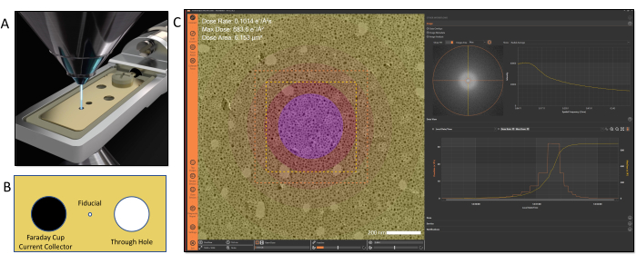
Figure 2: Electron dose calibration and tracking. (A) Dose is calibrated using a dedicated sample holder that contains a current collector positioned at the sample plane for beam current measurements. (B) Illustration of the features of the tip design: Left: Faraday cup; Middle: fiducial hole; Right: through hole (C). The applied electron dose can be visualized in the software using color-coded maps to denote different dose exposures within an image. Please click here to view a larger version of this figure.

Figure 3
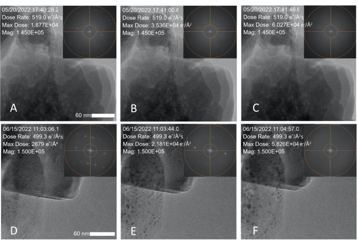
Figure 3: Electron dose induced degradation of zeolite (ZSM-5) nanoparticles. (AC) Snapshots taken over a 1 min and 20 s period showing degradation data obtained with a 300 kV FEG and a measured dose rate of 519 e2·s; the zeolite degrades within 1 min and 20 s. (DE) Snapshots taken over a 1 min and 50 s time period showing degradation data obtained with a 200 kV cold FEG TEM and an electron dose rate of 499 e2·s; the insets show the FFT spot fading over time. The scale bar is 60 nm. Please click here to view a larger version of this figure.

Figure 4
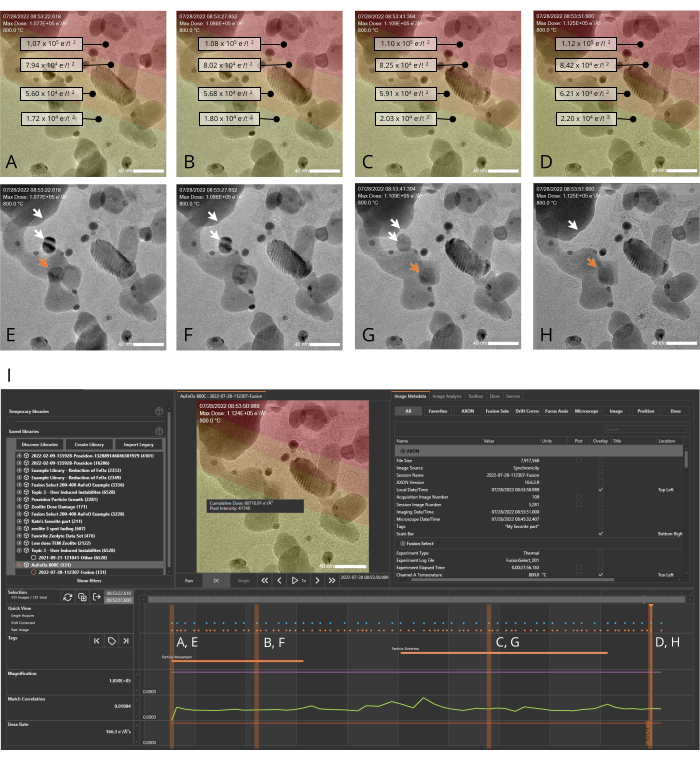
Figure 4: AXON synchronicity applies machine-vision algorithms to track and stabilize dynamically evolving samples. Metadata generated during the experiment can be plotted along the timeline, allowing the user to quickly pair an image with its associated metadata as they scroll through the image series generated during the experiment. (AH) Images of a nanocatalyst sample (Au/FeOx) at 800 °C recorded over a period of 28 s both with (AD) and without (EH) the dose map overlay. Red areas in the overlay indicate regions of high cumulative dose exposure, and yellow areas indicate regions of lower exposure. Highlighting an individual pixel indicates the cumulative dose for that pixel. White arrows in panels EH indicate two particles that merge during the experiment, and the orange arrow indicates the trajectory of a moving gold particle. (I) The experiment timeline generated by the analysis software for the image series shown in AH. The orange dots at the top of the timeline denote raw (non-digitally corrected) images and the blue dots denote drift corrected images. The orange vertical bars indicate the points on the timeline corresponding to the images shown panels AH. The scale bar is 40 nm. Please click here to view a larger version of this figure.

Figure 5
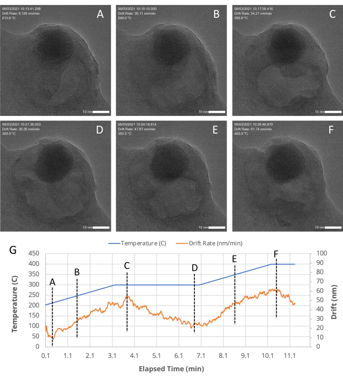
Figure 5: TEM snapshots of a porous region within an Au/FeOx nanocatalyst at various time points. The MVS software stabilizes and centers the sample even during high drift rates, such as those that occur during a temperature ramp through the application of stage, beam shift, and digital corrections, as indicated by machine-vision algorithms. (AF) TEM snapshots of a porous region within an Au/FeOx nanocatalyst, recorded at various (G) time points during an in situ heating experiment. The drift rate of the ROI is automatically calculated and recorded during an experiment by the MVS software. As plotted in (G), as the temperature profile is changed (the blue line), the drift rate (orange line) increases as the temperature increases and decreases as the temperature is held constant. Please click here to view a larger version of this figure.

Microscope Type 300 kV FEG TEM 200 kV Cold FEG TEM
Spot Size/Condenser 2 Aperture 3/100 µm 1/100 µm
Dose Rate 519 e/A2•s1 499 e/A2•s1
Loss of Structure Measured by FFT
(Accumulated Dose)
60,270 e/A2 58,230 e/A2

Table 1: Summary comparison of zeolite degradation results obtained from different microscopes.

Supplementary File 1: Screenshot of the MVS software interface with the dose management tab open. Please click here to download this File.

Supplementary File 2: MVS software database file of the beam-induced zeolite degradation experiment. This viewing/analysis software is available to download for free. Please see Supplementary File 9 for download instructions and computer specifications. Please click here to download this File.

Supplementary File 3: Movie of the beam induced zeolite degradation. Please click here to download this File.

Supplementary File 4: CSV file 1 (zeolite degradation: raw data [mechanical correction only]) Please click here to download this File.

Supplementary File 5: CSV file (zeolite degradation: drift corrected [mechanical + digital correction]) Please click here to download this File.

Supplementary File 6: MVS software database file nanocatalyst in situ heating experiment. Please click here to download this File.

Supplementary File 7: Movie of the nanocatalyst at 800 °C with dose overlays. Please click here to download this File.

Supplementary File 8: Movie of the nanocatalyst during a temperature ramp with coordinated drift values. Please click here to download this File.

Supplementary File 9: Instructions for downloading the free analysis software. Please click here to download this File.

List of Materials

ARM200F CFEG JEOL Transmission Electron Microscope (200 kV)
AXON DOSE Calibration Holder Protochips, Inc. AXA-FC-TFS Dose calibration and management hardware package for ThermoFisher ScientificTEM
AXON DOSE Software:  Version 10.6.5.3 Protochips, Inc. AX-MOD-DOSE-01-1YR Dose calibration and management software
AXON Studio Software: Version 10.6.5.3 Protochips, Inc. No Part Number.
Available to download at  success.protochips.com
Offline analysis software for AXON datasets.  A free copy of the AXON Studio software is available for down load at:  success.protochips.com
AXON Synchronicity Core Protochips, Inc. AXON-CORE Hardware component of the synchronization software.
AXON Synchronicity Software:  Version 10.6.5.3 Protochips, Inc. AX-MOD-SYNCPRO-01-1YR Synchronization software
Fusion In-Situ Heating E-chip Protochips, Inc. E-FHDC-VO-10 Sample Support E-chip with carbon film.  Used with in situ heating system
Fusion Select In Situ Heating System Protochips, Inc. FFAD-6200-EXP In-situ MEMs heating system for ThermoFisher Scientific TEM.
Gold(III) chloride (50% gold basis) hydrate 50790 Sigma Aldrich 27988-77-8 Used to prepare Au/FeOx nanocatalyst.  Coprecipitation synthesis procedure followed in C. Sze et al. Materials Letters. 36 (1–4), 11–16 (1998)
Iron (III) Oxide 310050 (Fe2O3) Sigma Aldrich 1309-37-1 Used to prepare Au/FeOx nanocatalyst.  Coprecipitation synthesis procedure followed in C. Sze et al. Materials Letters. 36 (1–4), 11–16 (1998)
Titan ChemiSTEM ThermoFisher Scientific Transmission Electron Microscope (300 kV)
Zeolite ZSM-5 Zeolyst CBV 8014  Nanocatalyst sample:  80 SiO2/Al2O3 Mole Ratio

Lab Prep

Transmission electron microscopy (TEM) enables users to study materials at their fundamental, atomic scale. Complex experiments routinely generate thousands of images with numerous parameters that require time-consuming and complicated analysis. AXON synchronicity is a machine-vision synchronization (MVS) software solution designed to address the pain points inherent to TEM studies. Once installed on the microscope, it enables the continuous synchronization of images and metadata generated by the microscope, detector, and in situ systems during an experiment. This connectivity enables the application of machine-vision algorithms that apply a combination of spatial, beam, and digital corrections to center and track a region of interest within the field of view and provide immediate image stabilization. In addition to the substantial improvement in resolution afforded by such stabilization, metadata synchronization enables the application of computational and image analysis algorithms that calculate variables between images. This calculated metadata can be used to analyze trends or identify key areas of interest within a dataset, leading to new insights and the development of more sophisticated machine-vision capabilities in the future. One such module that builds on this calculated metadata is dose calibration and management. The dose module provides state-of-the-art calibration, tracking, and management of both the electron fluence (e2·s-1) and cumulative dose (e2) that is delivered to specific areas of the sample on a pixel-by-pixel basis. This enables a comprehensive overview of the interaction between the electron beam and the sample. Experiment analysis is streamlined through a dedicated analysis software in which datasets consisting of images and corresponding metadata are easily visualized, sorted, filtered, and exported. Combined, these tools facilitate efficient collaborations and experimental analysis, encourage data mining and enhance the microscopy experience.

Transmission electron microscopy (TEM) enables users to study materials at their fundamental, atomic scale. Complex experiments routinely generate thousands of images with numerous parameters that require time-consuming and complicated analysis. AXON synchronicity is a machine-vision synchronization (MVS) software solution designed to address the pain points inherent to TEM studies. Once installed on the microscope, it enables the continuous synchronization of images and metadata generated by the microscope, detector, and in situ systems during an experiment. This connectivity enables the application of machine-vision algorithms that apply a combination of spatial, beam, and digital corrections to center and track a region of interest within the field of view and provide immediate image stabilization. In addition to the substantial improvement in resolution afforded by such stabilization, metadata synchronization enables the application of computational and image analysis algorithms that calculate variables between images. This calculated metadata can be used to analyze trends or identify key areas of interest within a dataset, leading to new insights and the development of more sophisticated machine-vision capabilities in the future. One such module that builds on this calculated metadata is dose calibration and management. The dose module provides state-of-the-art calibration, tracking, and management of both the electron fluence (e2·s-1) and cumulative dose (e2) that is delivered to specific areas of the sample on a pixel-by-pixel basis. This enables a comprehensive overview of the interaction between the electron beam and the sample. Experiment analysis is streamlined through a dedicated analysis software in which datasets consisting of images and corresponding metadata are easily visualized, sorted, filtered, and exported. Combined, these tools facilitate efficient collaborations and experimental analysis, encourage data mining and enhance the microscopy experience.

Procedura

Transmission electron microscopy (TEM) enables users to study materials at their fundamental, atomic scale. Complex experiments routinely generate thousands of images with numerous parameters that require time-consuming and complicated analysis. AXON synchronicity is a machine-vision synchronization (MVS) software solution designed to address the pain points inherent to TEM studies. Once installed on the microscope, it enables the continuous synchronization of images and metadata generated by the microscope, detector, and in situ systems during an experiment. This connectivity enables the application of machine-vision algorithms that apply a combination of spatial, beam, and digital corrections to center and track a region of interest within the field of view and provide immediate image stabilization. In addition to the substantial improvement in resolution afforded by such stabilization, metadata synchronization enables the application of computational and image analysis algorithms that calculate variables between images. This calculated metadata can be used to analyze trends or identify key areas of interest within a dataset, leading to new insights and the development of more sophisticated machine-vision capabilities in the future. One such module that builds on this calculated metadata is dose calibration and management. The dose module provides state-of-the-art calibration, tracking, and management of both the electron fluence (e2·s-1) and cumulative dose (e2) that is delivered to specific areas of the sample on a pixel-by-pixel basis. This enables a comprehensive overview of the interaction between the electron beam and the sample. Experiment analysis is streamlined through a dedicated analysis software in which datasets consisting of images and corresponding metadata are easily visualized, sorted, filtered, and exported. Combined, these tools facilitate efficient collaborations and experimental analysis, encourage data mining and enhance the microscopy experience.

Tags