All procedures abode by the Canadian Institutes of Health Research rules and were approved by the University of Montreal Animal Care and Use Committee.
1. Preparation of Rat Brain Slices
- Prepare 1 L of a sucrose-based solution (Table 1) and 1 L of standard artificial cerebral-spinal fluid (aCSF) (Table 2).
- Bubble the sucrose-based solution with a mix of 95% O2 and 5% CO2 (carbogen) for 30 min before placing it in -80 °C for about 30 min, until the solution is cold but not entirely frozen. Use this ice-cold sucrose as the cutting buffer for the slicing of the brain. Keep it on ice once it is removed from the freezer.
- Bubble the aCSF with carbogen through the entire experiment. Use this solution for slice storage and as the perfusing buffer in which the patch-clamping and biocytin-filling of astrocytes will be performed. Prepare a slice recovery holding chamber to deposit the brain slices as soon as they are cut.
Note: The slice recovery holding chamber could be custom-made and consists essentially of one small well with a mesh at the bottom suspended in a larger well that is filled with aCSF, in which a tube is inserted to bring carbogen from the bottom. - Use 15- to 21-day-old Sprague-Dawley rats without any sex- or strain-specific bias. Anesthetize the animal with isoflurane (1 mL of isoflurane in an anesthesia induction chamber). Check the depth of anesthesia by gently pinching the hind paw or tail of the animal.
- Decapitate the rat using a guillotine, cut its skull with scissors, and quickly remove the brain from the cranium with a flat spatula.
- Dip the brain in the ice-cold sucrose-based solution for about 30 s and transfer it (with the solution) to a petri dish. With a razor blade, remove the portions that are anterior and posterior to the area to be sectioned, if cutting slices in the transverse plane.
- Glue the remaining block of brain tissue on its rostral side and proceed to cut brain slices (350 µm thick) in the sucrose-based medium using a vibratome. Then, transfer the collected slices in a recovery holding chamber filled with carbogenated aCSF at room temperature (RT) until they are ready to be used (allow at least 1 hour for recovery).
Note: Recent developments in the field allow prolonged incubation up to 24 h of brain slices in in vitro conditions17.
2. Sulforhodamine 101 (SR-101) Labeling of Astrocytes
- Pre-heat a water bath to 34 °C and place two slice incubation chambers in it. Fill one of the slice incubation chambers with a solution of aCSF containing 1 μM SR-101, and fill the other only with aCSF.
- Incubate the slices in the incubation chamber containing the 1 µM SR-101 for 20 min and then transfer them into the second incubation chamber to rinse out excess SR-101 from the tissue. Let it incubate for 20 min or more at 34 °C, then keep the incubation chamber containing the slices at RT until they are needed18.
3. Astrocyte Patching and Biocytin Filling
- Select a slice and place it in the recording chamber of the microscope. To patch astrocytes, use electrodes with a resistance of 4-6MΩ when filled with a potassium-gluconate-based solution (see Table 3).
- Under visual guidance and using a micromanipulator, direct the recording electrode towards an SR-101-labeled astrocyte as shown in Figure 1. Avoid cells located at the surface of the slice since they are more likely to be damaged or have lost connections to neighboring cells.
- To prevent leakage of biocytin in the tissue, minimize the positive pressure added to the patch pipette and apply it only when it is close to the astrocyte that will be patched (0.1-0.4 mL in a syringe of 1 mL).
- Prior to patching, adjust the offset of the pipette and its capacitance. Correct for liquid junction potentials, as accurate and precise voltage commands are critical to the experiments19.
- Move the pipette close enough to the astrocyte to observe depression caused by the positive pressure. Then, remove the positive pressure and slowly apply some negative pressure. Clamp the astrocyte to -70 mV when the seal reaches 100 MΩ. Wait until the seal reaches 1-3 GΩ. Continue to apply negative pressure until breaking into the cell. Be careful while applying negative pressure, since astrocytes are very fragile.
- Assess the electrophysiological properties of the patched cell. In voltage-clamp mode, perform a whole-cell current-voltage protocol with a ramp voltage command of 600 ms duration ranging from -120 to +110 mV. In current-clamp mode, perform a step IV protocol in which the injection of 1000 ms current steps of 100 pA from -1 to 1 nA, the sampling rate of the whole-cell recordings is 10 kHz.
Note: Astrocytes show a linear current-voltage profile without any kind of rectification (as shown in Figure 1B) and no action potential firing upon membrane depolarization (Figure 1C). The resting membrane potential (RMP) should be stable and not positive to -60mV. In some brain areas, the RMP of astrocytes is more hyperpolarized than in the NVsnpr. - Allow the biocytin to diffuse within the astrocyte for 30 min while performing a step IV protocol every 5 min.
- Retract and detach the patch pipette carefully without damaging the patched astrocyte and immediately take note of the offset of the pipette before taking it out of the recording chamber. Subtract that value from the membrane potential recordings.
- Leave the brain slice to rest in the recording chamber for a minimum of 15 min (in addition to the 30 min for injection) to allow spreading of the tracer from the patched astrocyte to the entire network of coupled cells.
Note: To reveal a network of coupled cells, only a single cell should be patched in the nucleus of interest. If multiple attempts are required in order to achieve a successful patch, discard the case and try to patch on the contralateral side or in another brain slice. - Make a mark or incision in the tissue to identify which side of the slice is facing upwards, and transfer the slice first to a petri dish containing normal aCSF, then into a solution of 4% paraformaldehyde (PFA). Incubate the slice at 4 °C overnight.
CAUTION: PFA is extremely harmful. Use protective equipment in a ventilated hood. Ensure that all materials (brushes, tubes, etc.) that have been in contact with PFA do not contact the recovery holding chamber, incubation chamber, or other materials used for recording the fresh tissue.
4. Biocytin Revelation
- Revelation with fluorescent streptavidine
- Wash the brain slices 2 x 10 min in 0.1 M phosphate buffer saline (PBS) at RT. Then, reveal the biocytin by incubating the brain slices with streptavidine conjugated to a fluorophore at 1/200 dilution in PBS with 4% non-ionic detergent for 4 h at RT.
- Wash the brain slices 3 x 10 min in 0.1 M PBS at RT and mount the sections on glass slides using an aqueous mounting medium. Place the sides that were injected upwards, coverslip the slides, and seal them with nail-varnish.
- Revelation with DAB
Note: DAB (3,3-diaminobenzidine) revelation can be used when fluorescence cannot be used. In this case, only one revelation method should be employed for making comparisons.- Wash the brain slices 3 x 10 min in PBS at RT. Incubate the slices in PBS + H2O2 0.5% for 1 hour at RT.
- Rinse the slices 3 x 10 min in PBS at RT. Then, incubate the slices in an avidin-biotin complex staining solution composed of PBS and 0.1% non-ionic detergent + avidin-biotin complex peroxidase standard staining kit reagents at 1/100 for 24 hours at RT.
- Rinse the slices 3 x 10 min in PBS at RT, incubate them in a solution of PBS + DAB 0.05% for 20 min at RT, and transfer them into a solution of PBS + DAB 0.05% + H2O2 0.5%.
CAUTION: DAB is extremely harmful. Use protective equipment in a ventilated hood. The color reaction is stopped when the slices are transferred in PBS. - Rinse the slices 5 x 10 min in PBS at RT, mount the sections on glass slides (face the sides that were injected upwards) and let them dry on a slide drying bench overnight at 34 °C.
- Submerge the glass slides for 1 min in several alcohol baths at 70%, 95%, and 100%, and end with a bath of xylene for 1 min.
- Mount the glass slides using a toluene-based synthetic resin mounting medium. Place coverslips on the slides and seal them with nail varnish.
5. Network Imaging
- Visualize the astrocytic networks using a scanning confocal microscope equipped with 20X and 4X objectives (or an appropriate objective to visualize the entire nucleus where the network is located) and a laser to detect the fluorophore (in this case, Alexa-594 is used).
- Use the 20X magnification to make a z-stack of the network of labeled cells. Use a resolution of 800 x 800 pixels and scan speed of 12.5 μs/pixel.
Note: In order to image the whole network, multiple stacks are usually required, and the number of stacks needs to be adjusted for each network. The resolution and scan speed can be changed, but make sure to use the same settings to image all data. - Use the 4X magnification to take images of the network and region of interest.
Note: The 4X imaging is used to determine the network position within the nucleus of interest. Always image the same field in transmitted light. This image will be useful if you cannot determine the border of the nucleus in the confocal fluorescent image.
6. Image Analysis
- Data preparation
- Use the software ImageJFIJI (download it at https://fiji.sc/). Open the file and click OK in the “Bio-Formats Import Options” window.
- To redefine a z-stack that will contain only the optical slices needed for the final z-stack (Figure 2A), click on the “Stack” knob in the toolbar (to find, first select stk | Z Project). Select “Max Intensity” in the projection type setting (Figure 2A). Save the file and name it “stack file”.
- If the imaging file contains several channels, split it to conserve only the channel with the astrocytic network imaging (Image | Color | Split Channels).
- Check the pixel settings of the image [Image | Properties | Pixel (with "1" for pixel dimension)].
- Use the subtract background tool (Process | Subtract Background) to remove the background of biocytin labelling. Use the preview function to set the rolling ball radius, which is generally set at 50 pixels (Figure 2B).
- Use the remove outliers tool (Process | Noise | Remove Outliers) if it is required following the subtract background step. Select “Bright” in the “Which Outliers” setting (Figure 2C). Use the preview function to set the radius and threshold. Be careful with this tool, since it may blur the data, as shown in Figure 2D.
Note: This tool removes the small spots caused by unspecific deposits of streptavidine (as shown by the white arrows in Figure 2B and 2C before and after treatment, respectively). - Adjust the threshold (Image | Adjust | Threshold). Select “Default” and “B&W” mode (Figure 2E). Click on “Apply”.
Note: Auto-adjusting can be used, but manual adjusting with the two slider bars is preferred. The aim of this step is to reduce noise to the maximum without losing any labeled cells. - Convert the image into a binary image with the binary process tool (Process | Binary | Make Binary) as shown in Figure 2F. Save the file as a TIFF file and name it “binary file”.
- Cell counting
- Check the setting of the measure function (Analyze | Set measurement). Select the “Centroid” option.
- Use the “Analyze Particles” tool on the “binary file” (Figure 3A) produced in the previous step (Analyze | Analyze Particle) (Figure 3C on the left). Select “Outlines” in the “Show” setting (Figure 3C). This generates a new file that shows the result of the detection (Figure 3B).
- Play with the parameters: size (to detect only cells, use values between 30 and 6000) and circularity (to determine an interval between 0 to 1, in which “1” defines a perfect circle and “0” a random shape) to refine the detection (Figure 3C, left portion). Run the detection by clicking “OK”.
Note: Two tables will appear following the detection: 1) a table titled “Summary” that provides the number of detected cells, and 2) a table titled “Results” (Figure 3C, right portion) that provides the x- and y-coordinates of each cell. - Copy the values and paste them into a spreadsheet application. Save this table under the name “detection table”. A file with a plot of detected cells will also appear (Figure 3B). Save this file as a TIFF file under the name “detection file”.
- If a group of 2 or more labeled cells in the network are detected as a single cell with the analyze particles tool because they are too close to each other, use the watershed tool (Process | Binary | Watershed) on the binary image before applying the analyze particles tool, and redo the analyze particles steps.
Note: The watershed tool creates a delimitation of 1 pixel wide between extremely close cells. A cell counter plug-in can be used when labeling is unequivocal and can be conducted manually.
- Measuring astrocytic network area
- To measure the surface area of the networks, use the detection file using Image J.
- Use the polygon selection tool (left click on the button in the tool bar to select it) to trace a polygon that connects all the cells located in the external periphery of the network (Figure 4A). Left click to begin tracing the polygon, and right click to close it.
Note: This polygon will be defined as a region of interest (ROI) and its surface will be measured to determine the surface area of the network. - Open the set measurement window (Analyze | Set Measurement) and select the “Area” option. Open the ROI Manager (Analyze | Tools | ROI Manager) (Figure 4B). Then, add the traced polygon in the ROI Manager by clicking ‘’Add’’ (Figure 4B) and run the measurement by clicking ‘’Measure’’ in the ROI Manager.
Note: The area measurement will appear in a table and be expressed in pixels. Do not forget to convert this value with the conversion factor for the microscope used to obtain a value in μm2.
- Determination of the main direction vector
- Determination of the patched cell
- Open the stack file in ImageJFIJI and identify the patched cell in the stack file based on its stronger labeling intensity (Figure 4C). Then, open the file named “detection table” in a spreadsheet application and find the number associated to the patched cell and its corresponding coordinates.
- If unable to accurately determine the patched cell, surround the area where the deposit of biocytin is denser in the imaged network of coupled cells, using the Polygon tool in ImageJFIJI, and refer to this position as that of the patched cell (Figure 4D).
- Use the ROI Manager (Analyze | Tools | ROI Manager). Then, draw a ROI at the patched cell location and add it to the ROI Manager (see Figure 4B).
- Set a measurement (Analyze | Set Measurement) and select the “Centroid” option.
- In the ROI Manager, click on “Measure” to obtain the coordinates of the centroid of the traced area. Use these coordinates as the reference point for this specific network.
- Referential translation
- Calculate the coordinates of each cell in reference to the patched astrocyte by using the following formula:

With: as the coordinates for a given cell;
  as the coordinates of the patched cell (or the referential point of the network); and
  as the coordinates for a given cell in the new referential.
Note: Expressing the coordinates of each cell in reference to the patched astrocyte is an important step in calculating vectors from the patched astrocyte. Be careful when using ImageJFIJI that the referential for any image is located in the top-left corner of the image.
- Calculate the coordinates of each cell in reference to the patched astrocyte by using the following formula:
- Determination of the main vector of preferential orientation
- Calculate the coordinates of the main vector of preferential orientation with the following formula:

With: ( ) as the coordinates of the main vector of preferential orientation; and
 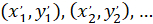 as the coordinates of each cell of the network obtained with the patched cell as referential.
Note: For each cell in the network, a vector is determined relative to the coordinates of the patched astrocyte. The main vector of preferential orientation of the network is the sum of all these vectors. - Divide the length of the main vector (provided by the coordinates obtained from using the above formula) by the number of cells in the network minus one (since the coordinates of the patched cell are not included), to normalize the values and enable comparisons between networks. A schematic view of this analysis is presented in Figure 5.
- Calculate the coordinates of the main vector of preferential orientation with the following formula:
- Determination of the patched cell
- Placement of analyzed networks in the nucleus of interest
- Alignment of the 20X and 4X images
- To determine the position of each network in the nucleus of interest (NVsnpr), use the 4X image. Open the 4X image with a vector image editor.
- Select the 4X image and modify its size by multiplying it by 5. The dimension window is located in the right part of the top horizontal toolbar. For instance, for a 4X image that has been sampled at 800 x 800 pixels, change the sampling resolution to 4000 x 4000 pixels (to set the working unit in pixels, go to “Document Setup” under the file tab: File | Document Setup). Export the file in TIFF format and name it “resized 4X”.
- Align the top-left corner of the image with the bottom-left corner of the Adobe Illustrator document.
Note: The software provides coordinates from a bottom-left corner referential point. - Open the 20X image of the network. Use the ‘’binary file’’ or ‘’detection file’’ because they are easier to align. Then, play with the opacity tool on the ‘’binary file’’ of the 20X image to align it with the re-sized 4X image.
Note: The opacity tool is in the top horizontal tool bar. - When the alignment is done, select and hold the pipette tool so the measure tool appears, and select it in the left toolbar.
- Use the measure tool to click on the top-left corner of the 20X image to get the coordinates of the 20X referential point onto the resized 4X image.
Note: These coordinates, which are referred to as the 20X referential (20XR in Figure 5), will be useful for expressing the position of each network on a schematic drawing of the nucleus.
- Normalization of the nucleus of interest
Note: To sum up the data, a normalization of the nucleus (NVsnpr) as a rectangle is used. The steps are described below.- Open the 4X resized file in ImageJFIJI, and use the polygon tool to surround the nucleus (NVsnpr). Use the image with transmitted light if the borders of the nucleus are not able to be seen; in which case, remember to resize it first.
- Open the ROI Manager and add the drawn ROI. In “Set Measurement”, select the ‘’Bounding Rectangle’’ option.
Note: The “Bounding Rectangle” option calculates the smallest rectangle around the drawn nucleus. - Click “Measure”.
Note: A table appears with BX and BY, the coordinates of the top left corner of the rectangle: ‘’Rectangle Position’’ and provides the width and height. BX and BY are the coordinates of the bounding rectangle referential which are referred to as and
and  .
.
- Expression of each network position in the normalized nucleus
- Express the coordinates of each cell with the 4X referential (black square in Figure 5) using the following formula:

Where: are the cell coordinates with the 4X referential;
  are the cell coordinates with the 20X referential (orange square in Figure 5); and
  are the coordinates of the 20X referential point in the 4X image (20XR).
 - Express the cell coordinates in the bounding rectangle referential (blue in Figure 5) using the following formula:

Where: are the cell coordinates in the bounding rectangle referential;
  are the cell coordinates in the 4X referential; and
  are the coordinates of the bounding rectangle referential in the 4X image.
 - Transform the cell coordinates in the bounding rectangle referential to the percentage of width and height of the bounding rectangle using the following formula:
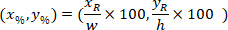
Where: are the cell coordinates in the percentage of width and height of the bounding rectangle;
  are the cell coordinates in the bounding rectangle referential;
  is the width of the bounding rectangle measured above in the protocol; and
  is the height of the bounding rectangle measured above in the protocol.
 - To represent all the networks on the same figure, take into account the orientation of the slice (left or right side). To standardize the data, the referential is applied on the left side of the slice. Transfer the network coordinates of the right side to the left side by applying the following formula only to x-coordinates:

Where: is the x-coordinate on the right side of the slice; and
  is the new x-coordinate expressed in the referential on the left side of the slice.
Note: Alternatively, mirror the picture in ImageJFIJI before the analysis (Image | Transform | Flip Horizontally). - To express the coordinates of the main vector of preferential orientation, follow the same steps with the cell coordinates (steps 6.5.3.1 to 6.5.3.4).
Note: The expression of the coordinates in percentages allows a compilation of the data as a single plot in which the nucleus (NVsnpr) is designed as a rectangle.
- Express the coordinates of each cell with the 4X referential (black square in Figure 5) using the following formula:
- Alignment of the 20X and 4X images
- Study of the angular difference of the main vector of preferential direction
Note: The angular difference of an astrocytic network is used to determine whether its preferential orientation is towards the center of the nucleus of interest. To calculate the angular difference (α in Figure 5), which is the angle between the main vector of preferential direction of the network (PD, red line in Figure 5) and the line connecting P to C, apply the Al-Kashi Theorem into the triangle PDC (see inset of Figure 5 and Supplementary Methods).- First, calculate the different lengths using the application of the Pythagorean Theorem into a Cartesian referential using the following equation:
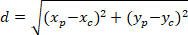
Where: the coordinates of P and C are and
and  , respectively, in the bounding rectangle referential (calculated above).
 - Determine the angular difference in radians using the following formula:
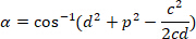
- Convert the angular difference in degrees (e.g., with the DEGREES function in Excel software).
- Compile all the angular differences by plotting them in vertical bar charts (Figure 7C and 7D) and determine if there is a preferential orientation of astrocytic networks.
- First, calculate the different lengths using the application of the Pythagorean Theorem into a Cartesian referential using the following equation:
Coupling between cells in the brain is not static but rather dynamically regulated by many factors. The methods described were developed to analyze astrocytic networks revealed under different conditions and to understand their organization in NVsnpr. These results have been already published1. We performed biocytin filling of single astrocytes in the dorsal part of the NVsnpr in three different conditions: at rest (in control conditions in the absence of any stimulation), in Ca2+-free conditions, and following the electrical stimulation of sensory fibers that project to the nucleus. The experimental settings for the biocytin filling of astrocytes for each condition are illustrated in the left sides of Figure 6A-C.
Networks of biocytin-labeled cells were observed in control conditions and confirmed a basal state of cell coupling between NVsnpr astrocytes at rest. In 11 tested cases, biocytin diffusion showed networks composed of 11 ± 3 cells (middle panel in Figure 6A, Figure 6D) extending over an area of 34737 ± 13254 µm2 (Figure 6E). Carbenoxolone (CBX, 20 μM), a non-specific blocker of gap junctions, was used in an independent set of experiments to ensure that the observed labeling was a result of biocytin diffusion through gap junctions and not uptake by the cells of biocytin, which could leak into the extracellular space from the positive pressure applied to the patch pipette prior to patching. Bath application of CBX reduced the number of labeled cells to 2 ± 0.5 cells (right panel in Figure 6A, Figure 6D; Iman-Conover method, P = 0.016; Holm-Sidak test, P = 0.010) and the area of biocytin spread to 2297 ± 1726 µm2 (Figure 6E; Iman-Conover method, P = 0.0009; Holm-Sidak test, P = 0.025).
The effect of calcium removal from the medium on the NVsnpr astrocytic networks was tested because low extracellular calcium concentration is known to open connexins and gap junctions20,21,22, and it can be used as a massive and uniform stimulus to open up the syncytium and maximize tracer diffusion through gap junctions. The astrocytic networks that were revealed in Ca2+-free conditions (n=10) showed a larger number of cells than the networks revealed in control conditions, with 37 ± 10 labeled cells (middle panel in Figure 6C, Figure 6D; Iman-Conover method, P = 0.016; Holm-Sidak test, P < 0.001) covering an area of 108123 ± 27450 μm2 (middle panel in Figure 6C, Figure 6E; Iman-Conover method, P = 0.009; Holm-Sidak test, P = 0.001).
Compared to the complete removal of calcium from the medium, electrical stimulation of afferent inputs to the nucleus of interest is a more physiological stimulus that directly involves the neuronal circuitry of interest. Consequently, the results from this type of manipulation can provide meaningful information regarding the functional implications of the astrocytic networks observed. For instance, input from two different pathways may lead to different effects on the basal state of cells coupling in a given area, or it may elicit coupling between astrocytes in distinct subdivisions of the nucleus. In our circuit, electrical stimulation of the sensory fibers that project to the NVsnpr using 2-second trains of 0.2 ms pulses at 40-60 Hz (n = 11) produced an increase of the coupling between NVsnpr astrocytes, relative to the unstimulated conditions, with 23 ± 6 cells (middle panel in Figure 6B, Figure 6D; Iman-Conover method, P = 0.016; Holm-Sidak test, P = 0.012) spreading out over an area of 814174 ± 15270 μm2 (middle panel in Figure 6B, Figure 6E; Iman-Conover method, P = 0.009; Holm-Sidak test, P = 0.004).
The effects of these two types of stimulation, the removal of calcium from the medium, and the electrical stimulation of afferent inputs, are all disrupted by CBX. The astrocytic networks in this condition comprised only 5 ± 1 cells in Ca2+-free aCSF (right panel in Figure 6C, Figure 6D; n = 4; Iman-Conover method, P = 0.016; Holm-Sidak test, P < 0.001) and 9 ± 2 cells with sensory fibers stimulation (right panel in Figure 6B, Figure 6D; n = 6; Iman-Conover method, P = 0.016; Holm-Sidak test, P = 0.023). The network surface areas were also reduced to 17987 ± 9843 µm2 with Ca2+-free aCSF (Figure 6E; n = 4; Iman-Conover method, P = 0.009; Holm-Sidak test, P = 0.004) and to 39379 ± 11014 µm2 with sensory fibers stimulation (Figure 6E; n = 6; Iman-Conover method, P = 0.009; Holm-Sidak test, P = 0.055).
Anatomical analysis was performed only in cases where the NVsnpr boundaries could be clearly defined on 4X imaging, which was the case for 9 out of 10 networks obtained with Ca2+-free aCSF and 8 out of 11 networks obtained with electrical stimulation. Plotting of all the analyzed astrocytic networks on a theoretical NVnspr shows that most cells comprised in the networks were confined within the nucleus boundaries (Figures 7A and 7B, left and middle panels). Under Ca2+-free aCSF, 4 out of 9 astrocytic networks spread outside of the NVsnpr in the direction of the motor nucleus located medially to the NVsnpr. In these 4 cases, the vast majority of the labeled cells were confined to the nucleus. The networks of labeled cells obtained with electrical stimulation of the sensory fibers were more restricted. Only 2 networks extended over the nucleus borders, in which one spread over the mediodorsal border into the lateral supratrigeminal area (dark green network in Figure 7B, left and middle panels). In the second case, 2 astrocytes in the red network (Figure 7B, left and middle panels) crossed into the ventral portion of the NVsnpr.
The vectorial analysis for the astrocytic networks preferential orientation (right panel in Figure 7A and 7B) produced different results depending on the stimulus used. Indeed, for the astrocytic networks observed with Ca2+-free aCSF, all except one of the vectors of preferential orientation were oriented towards the center of the NVsnpr. However, for the astrocytic networks observed with electrical stimulation, the preferential orientation vectors were mostly oriented towards the borders of the nucleus. This is reflected by the computed angular differences in preferential orientation between the astrocytic networks obtained with Ca2+-free aCSF and those obtained with electrical stimulation of the sensory fibers. Under Ca2+-free aCSF, the vertical bar charts of the distribution of angular difference showed that most of the networks of labeled cells have an angular difference between 0 and 40 degrees, with a mean of angular difference of 39.5 ± 12.7 degrees (Figure 7C). With electrical stimulation of sensory fibers, the distribution is more uniform, and the mean angular difference (99.5 ± 17 degrees) is significantly different (Figure 7D; student t-test, P = 0.012).
These data show that biocytin labeling analysis allows us to distinguish the effects of different stimuli modulating astrocytic coupling. Moreover, mapping of the astrocytic networks in a normalized nucleus followed by vectorial analysis provides valuable information on the size and anatomical organization of these networks.
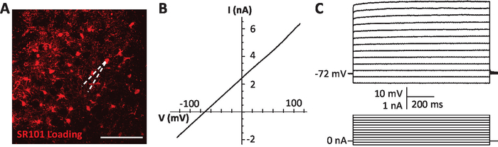
Figure 1: Whole-cell patch-clamp of astrocyte. (A) Astrocytes labeled with a loading of the marker sulforhodamine 101 (SR-101) in NVsnpr. An SR-101-labeled astrocyte soma is targeted with the patch pipette (white dashed line). Scale bar = 100 μm. (B) A depolarizing ramp protocol is performed in voltage-clamp (from -120 to 110mV) to assess the astrocyte passive characteristics. (C) Assessment of the lack of action potential firing in the astrocyte by injection of current pulses in current-clamp mode. This figure is adapted from Condamine et al. (2018)1. Please click here to view a larger version of this figure.
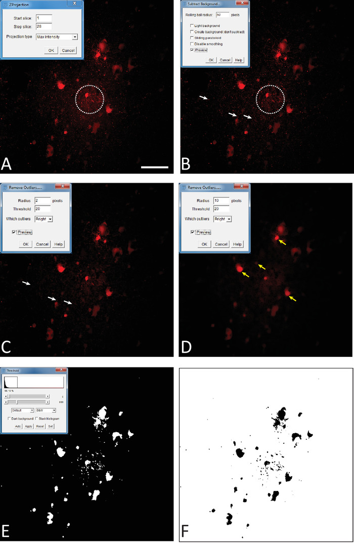
Figure 2: Treatment and analysis of astrocytic networks with ImageJFIJI software. (A) Z-Stack creation from the confocal imaging of an astrocytic network. At the top-left, Z-stack window in ImageJFIJI. (B) Background subtraction process. At the top-left, subtract background window in ImageJFIJI. The dotted circle emphasizes the area on the image where the effect of the subtract background command is the more obvious when compared to the image in A. (C) Remove outliers process. This process removes the small spots due to unspecific deposits of streptavidine coupled to an Alexa 594. The white arrows show the deposit prior to (Figure 2B) and after (Figure 2C) the command has been processed. In the top-left, remove outliers window in ImageJFIJI. (D) Example of the blurring effect that may be produced by an inadequate adjustment of the remove outliers parameters. Yellow arrows show some blurred cells. (E) Adjust threshold process. At the top-left, adjust threshold window in ImageJFIJI. The scroll bars act on the threshold signal adjustment. (F) Make binary step. The image is converted into a binary file in ImageJFIJI. Scale bar = 100 μm. Please click here to view a larger version of this figure.
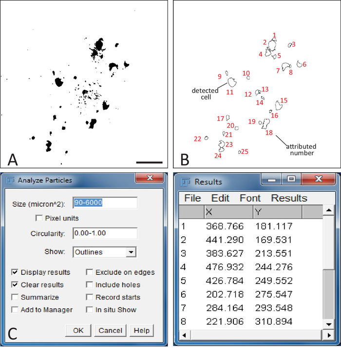
Figure 3: Detection of cells in astrocytic networks with ImageJFIJI. (A) Example of a binary image of an astrocytic network obtained in ImageJFIJI. Scale bar = 100 μm. (B) Illustrates the "detection file" obtained after applying the analyze particles process on the binary file. The shapes correspond to all the detected cells with their associated number in red. (C) Left part: analyze particles window in ImageJFIJI. This function detects the cells of the network in the binary image. The size of the detected cells and their circularity can be adjusted. Numbers to be used should be set by trial-and-error until a satisfactory result is obtained. Right part: detection table generated by the analyze particles process. X and Y columns list the coordinates of each cell detected in the image. Please click here to view a larger version of this figure.
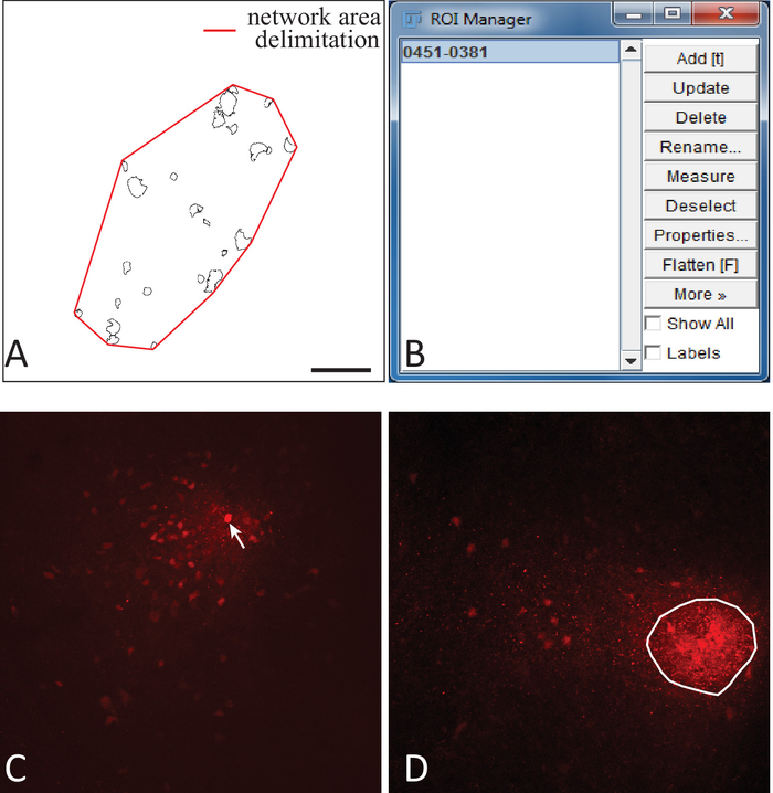
Figure 4: Network area analysis and determination of the patched cell in ImageJFIJI. (A) Using the polygon tool in ImageJFIJI, an ROI is traced around the cluster of detected cells (red line) that will be used to determine the surface area of the network. (B) The ROI is added into the ROI Manager. (C) Example of an astrocytic network in which the patched cell (white arrow) is easily identifiable because of the striking intensity of its biocytin labeling. (D) Example of an astrocytic network where the patched cell could not be identified, but where an area of denser labeling clearly indicates biocytin deposits. An ROI is drawn around this area and added to the ROI manager. Its centroid is computed and considered as the position of the patched cell to use for vectorial analysis. Scale bar = 100 μm. Please click here to view a larger version of this figure.
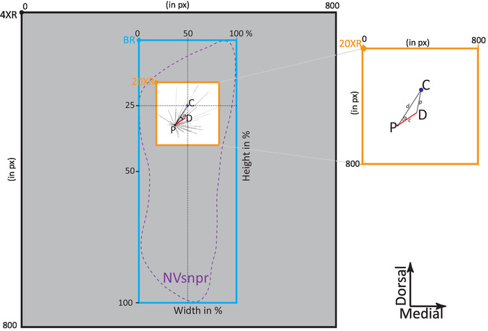
Figure 5: Diagram of the different referentials used for astrocytic networks analysis. The grey square is the 4X image with the referential point 4XR to be aligned with the left bottom corner of the Adobe Illustrator document. The white square surrounded in orange is the 20X image with the referential point 20XR. Both images are aligned with each other as described in the protocol. The bounding rectangle (blue) defines NVsnpr (purple dashed line) and is scaled in percentage with the referential point (BR). The theoric center of the dorsal part of NVsnpr is schematized by the dark blue dot (C). The astrocytic network is schematized by the patched cell (black dot, P) and the main vector of the preferential direction (red line). Each dashed black line is the vector of each cell of the astrocytic network. The angular difference of the astrocytic network (α) is the angle between the main preferential orientation of the network (red line) and the black line that connects the patched astrocyte to the theoretical center of the nucleus. Inset is a zoom of the 20X image showing the triangle PCD formed by the theoretical center of the NVsnpr (C), the patched cell, and the main vector of preferential direction (D). Please click here to view a larger version of this figure.
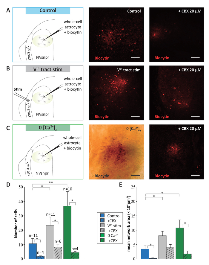
Figure 6: Astrocytic networks labeled with biocytin in NVsnpr under different conditions showing different sizes. (A-C) To the left, a schematic drawing of the experimental condition. In all conditions, a single astrocyte labeled by SR-101 was targeted for whole-cell recording and filled with biocytin (0.2%). Middle column: photomicrographs illustrating the astrocytic networks obtained under control conditions (A), after electrical stimulation of the Vth tract (2 s trains, 40-60 Hz, 10-300 µA, 0.2 ms pulses) (B); and after perfusion with a Ca2+-free aCSF (C). Right column: photomicrographs illustrating the astrocytic networks obtained under the same conditions but in the presence of CBX (20 μM) in the bath prior. Scale bar = 100 μm. (D and E) Vertical bars chart representing the number of coupled cells and the surface area, respectively, of the biocytin-filled networks of astrocytes under the three experimental conditions presented above (A, B, and C) in the presence (hatched) and absence (solid) of CBX (20 µM). Data are represented as mean ± SEM. Multiple comparisons (Holm-Sidak test): * = P < 0.05; ** = P < 0.001. This figure is adapted from Condamine et al. (2018)1. Please click here to view a larger version of this figure.
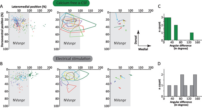
Figure 7: Characterisation of networks in NVsnpr under Ca2+-free aCSF and with electrical stimulation of the Vth tract. (A and B) Left: All cells labeled in 9 networks filled under perfusion with Ca2+-free aCSF (A) or in 8 networks filled while stimulating the Vth tract (B) are plotted according to their position in a theoretical NVsnpr nucleus (gray rectangle). Each network (and the cells composing it) is represented by a different color. Middle: Boundaries of each network. The dot in each area represents the patched cell. Right: Representation of main vector of preferential orientation of each network. The dot represents the patched cell and the arrow the vector of preferential direction. (C and D) Distribution of angular differences between the main vector of the preferential orientation and a straight line connecting the patched cell to the center of the dorsal part of NVsnpr (located at 25% on the dorsoventral axis and 50% on the mediolateral axis) under the two conditions studied. The mean angular difference was 39.5 ± 12.7 degrees in Ca2+-free aCSF, indicating a preferential orientation towards the centre of the nucleus and 99.5 ± 17 degrees with electrical stimulation, indicating a preferential orientation towards the periphery (student t-test, P = 0.012). This figure is adapted from Condamine et al. (2018)1. Please click here to view a larger version of this figure.
| sucrose-aCSF* | mMol |
| Sucrose | 219 |
| KCl | 3 |
| KH2PO4 | 1.25 |
| MgSO4 | 4 |
| NaHCO3 | 26 |
| Dextrose | 10 |
| CaCl2 | 0.2 |
Table 1: Composition of the sucrose-based solution used for brain slicing. (*) = pH and osmolarity were adjusted to 7.3-7.4 and 300-320 mosmol/kg, respectively.
| aCSF* | mMol |
| NaCl | 124 |
| KCL | 3 |
| KH2PO4 | 1.25 |
| MgSO4 | 1.3 |
| NaHCO3 | 26 |
| Dextrose | 10 |
| CaCl2 | 1.6 |
Table 2: Composition of the aCSF solution used for slice storage and whole-cell recording. (*) = pH and osmolarity were adjusted to 7.3-7.4 and 290-300 mosmol/kg, respectively.
| Internal patch solution* | mMol |
| K-gluconate | 140 |
| NaCl | 5 |
| HEPES | 10 |
| EGTA | 0.5 |
| Tris ATP salt | 2 |
| Tris GTP salt | 0.4 |
Table 3: Composition of the internal solution used for whole-cell recording. (*) = pH and osmolarity were adjusted to 7.2-7.3 and 280-300 mosmol/kg, respectively.
