Spatio-temporal control of actin regulatory proteins is associated with filopodium dynamics 1,2. Tracking spatially resolved protein concentration along the whole filopodial length through time is thus crucial to advance our understanding of the mechanisms underlying initiation, elongation, stabilization or collapse of these dynamic structures 3,4. Unlike protein analysis in the cytosol, where many cell shape changes occur at a larger scale, filopodia are dynamic micro structures that constantly buckle 5 and bend, thus precluding analysis using a simple approach such as a line-scan.
Different software solutions for tracking filopodial shape are available 6,7,8,9. Likewise, software for ratiometric tracking of protein dynamics within the cell body has been developed 10,11. To combine automated tracking of filopodial shape and spatio-temporal protein analysis, we recently developed an image analysis software based on the convex-hull algorithm 12. This novel analysis method, which is operated via a graphical user interface (GUI), combines for the first time, relative protein concentration along the filopodial length and growth velocity, thus allowing the accurate measurement of spatio-temporal protein distribution independent of movement of these dynamic structures 12.
The idea behind the software (source code is freely available, see below) is that one of the vertices of the convex hull will coincide with the tip of the filopodium (Figure 1A). By looking in the subsequent frame for the nearest vertex of the convex-hull, the moving tip can be tracked throughout the whole movie. Once the tip is detected in each frame, its position is used to draw an axis by joining the tip with a reference point at the base of the filopodium (Figure 1B). Finally, using equidistant nodal points, whose positions are determined by the median pixel with maximum intensity along the line orthogonal to the axis, are used to determine a backbone that follows the filopodial shape. Taking advantage of this adaptive backbone, a kymograph is generated to trace filopodial growth and protein concentrations for up to three channels along the filopodial length (Figure 1C).
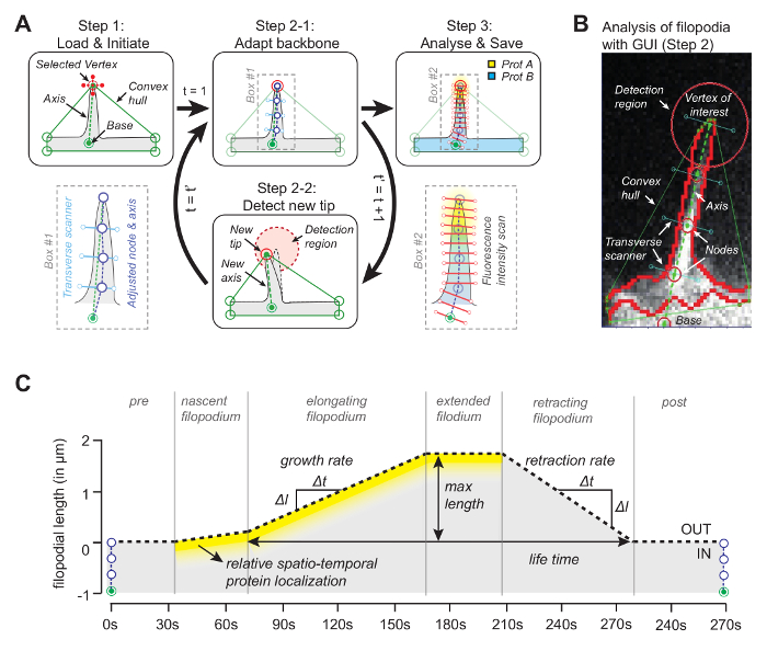
Figure 1: Working Principle of the Image Analysis Software. (A) The algorithm behind the software. In Step1 the user specifies the reference (base) and the vertex (the tip) of the filopodium. In Step 2-1 the backbone of the filopodium is obtained using the median pixel with maximum intensity value. In Step 3 the backbone is used for spatial protein intensity profile. In Step 2-2 the software automatically tracks the tip in the subsequent frame. The whole procedure iterates. (B) Snapshot of the algorithm with real filopodium introducing important elements such as the convex hull that is being used for tracking. (C) Overview of parameters that can be measured with the algorithm. This figure has been modified from reference 12. Please click here to view a larger version of this figure.
The image analysis software is operated in Matlab (referred to as programming software) via a graphical user interface. To maximize flexibility and robustness for the particular experimental setting, the user can adjust a series of tracking parameters (e.g. permitted bending angle and inter-frame movement) and also make some corrections to the movies (e.g. cropping, rotation, removal of unwanted objects) (Figure 2A and Table 1).
| GUI | No. | Mandatory | Description | Name (in GUI) | ||||
| #1 | 1a | Y | Loading stacked .tiff file representing cell body (with box checked in) or create superimposed cell body from channels | CellBody | ||||
| #1 | 1b | Y | Loading stacked image file corresponding to protein 1 | Protein 1 | ||||
| #1 | 1c | Y | Loading stacked image file corresponding to protein 2 | Protein 2 | ||||
| #1 | 1d | Y | Loading stacked image file corresponding to protein 3 | Protein 3 | ||||
| #1 | 1e | N | Resets everything to preloaded stacked image files | Reset | ||||
| #1 | 2a | Y | Scroll bar to determine the initial frame for analysis in GUI window #2 | NA | ||||
| #1 | 2b | Y | Scroll bar to determine the final frame for analysis in GUI window #2 | NA | ||||
| #1 | 2c | Y | Scroll bar representing current frame | NA | ||||
| #1 | 2d | N | The grey value of the pixels below which all pixels will be set to zero | NA | ||||
| #1 | 2e | N | The grey value of the pixels above which all pixels will be set to maximum values | NA | ||||
| #1 | 2f | N | Set the intensity values of the pixels specified by <2e> & <2f> | Set | ||||
| #1 | 2g | N | Play the intensity-adjusted movie | Play | ||||
| #1 | 2h | N | Crop Image | Crop | ||||
| #1 | 2i | N | Rotate Image | Rotate | ||||
| #1 | 2j | N | Delete regions in the whole stack | Delete regions | ||||
| #1 | 3a | Y | Click to open the ‘Analysis Window’ (GUI window #2) | Tracking Window | ||||
| #1 | 3b | Y | Enter the size of a pixel in microns | Enter Pixel size | ||||
| #2 | 4 | Y | Click to generate the boundary/edge image of the superimposed cell body | Boundary | ||||
| #2 | 5 | Y | Click to select the base and tip of the filopodia | Referernce | ||||
| #2 | 6a | Y | Enter the number of segments or nodes | No of segments | ||||
| #2 | 6b | Y | Enter the scan length (perpendicular to axis) | Scan Width | ||||
| #2 | 6c | Y | Enter the length above which filopodia starts bending | Accurate Meas after | ||||
| #2 | 6d | Y | Enter the radius of the tip detection circle (i.e. area where the vertex can be localized in the next frame) | Radius of tip detection | ||||
| #2 | 6e | Y | Enter the maximum angle the filopodium can bend from the vertical axis | Angle Threshold | ||||
| #2 | 6f | N | Add reference points for base and tip for that specific frame | Select reference | ||||
| #2 | 6g | N | Enter the length above which filopodia starts bending for that specific frame | Accurate Meas after | ||||
| #2 | 6h | N | Enter the radius of the detection circle for that specific frame | Radius of tip detection | ||||
| #2 | 6i | N | After entering all the parameters for the specific frame click to store the values to memory and file for further reference | Add | ||||
| #2 | 6j | N | Click to delete the set manually parameters for that frame | Delete | ||||
| #2 | 6k | N | Click to delete all parameters stored manually using the ‘optional features panel’ for all frames | Reset | ||||
| #2 | 6l | N | Check in before tracking to store all tracking results in memory for future reference | History trace | ||||
| #2 | 7 | Y | Click to start tracking | Track&Analyze | ||||
| #2 | 8a | N | Click to start tracking protein channel intensity | Analyze Protein Intensities | ||||
| #2 | 8b | N | Check in to track protein channel intensity along the filopodial length | Whole filopodia | ||||
| #2 | 8c | N | Check in for tracking the reference protein or protein A | ProteinA | ||||
| #2 | 8d | N | Check in for tracking the protein B | ProteinB | ||||
| #2 | 8e | N | Check in for tracking the protein C | ProteinC | ||||
| #2 | 8f | N | Check in to track average protein intensity in the tip | Leading tip | ||||
| #2 | 8g | N | Enter the length of the tip | Tip Length | ||||
| #2 | 8h | N | Enter the minimum distance from base above which the tip starts forming | threshold | ||||
| #2 | 8i | N | Click to save the leading tip analysis results to file | Push Button | ||||
| #2 | 9a | N | Click to initiate ratiometric protein analysis | Compare | ||||
| #2 | 9b | N | Check in to compare protein B with respect to A | log10(B/A) | ||||
| #2 | 9c | N | Check in to compare protein C with respect to A | log10(C/A) | ||||
| #2 | 9d | N | Check in to compare protein B with respect to A at the tip | log10(B/A) | ||||
| #2 | 9e | N | Check in to compare protein C with respect to A at the tip | log10(C/A) | ||||
| #2 | 10a | N | Choose other color-map (default: Jetplot) | Color Map | ||||
| #2 | 10b | N | Edit the colormap | Edit colormap | ||||
Table 1: Overview of All Functions Present in the GUI Windows #1 and #2.
Once this is accomplished, the program creates a convex hull and automatically tracks the tip throughout the movie. Parameters extracted from the movie, such as a ratiometric kymograph, growth velocity, and filopodial length are displayed and also stored in the work folder as images and as data files. Other parameters such as filopodial lifetime, growth rate and retraction rate can then be extracted and further analyzed from the stored data files (Figure 2B).
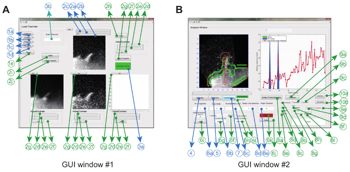
Figure 2: Graphical User Interface for using the Image Analysis Software. (A) GUI Window #1 is used for loading and processing images. The program can load up to 3 protein channels, whereby 2 channels are compared pair-wise. The window comes with mandatory (blue) and optional features (green) for pre-processing the images prior to tracking (B) GUI Window #2 is used for tracking the filopodium as well as spatio-temporal and ratio-metric protein analysis. Again, optional features are marked in green. This figure has been modified from reference 12. Please click here to view a larger version of this figure.
Here, we present a detailed protocol for sample preparation and software handling. We start with detailed instructions on culturing cells and acquiring movies optimized for image analysis. This section on data acquisition is followed by a detailed description for operating the image analysis software. Throughout the protocol, we introduce critical steps and optional features that should be considered when collecting and processing data. Finally, we analyze filopodia from different model systems with the image analysis software, before closing with a comparison of the described image analysis software with other programs available for filopodial quantification and a discussion on limitations and future direction.
1. Cell Culture
- Culture HeLa or COS cells in Dulbecco's Modified Eagle Medium (DMEM) containing 4.5 g/L D-glucose, L-alanine-L-glutamine dipeptide, pyruvate, 10% fetal bovine serum, and 10 units/ml of penicillin/streptomycin. Culture neurons in culture-media without L-glutamine, glutamic acid or aspartic acid, supplemented with 0.5 mM L-alanine-L-glutamine dipeptide, serum-free neuronal supplements and 10 units/ml of penicillin/streptomycin.
- Once 40% confluency is reached, transfect cells with constructs of choice using a transfection reagent as per manufacturer's instructions. Keep transfected cells in incubator at 37 °C and 5% CO2 for 15-18 h.
- To reduce changes in pH and osmolarity (due to evaporation) during image acquisition, fill the cell culture chambers (prior to imaging) up to 90 % with 37 °C pre-warmed medium containing 20 mM 4-(2-hydroxyethyl)-1-piperazineethanesulfonic acid (HEPES). To seal the lid, apply a thin layer of vacuum grease on the inside of the lid and gently press it on the culture chamber containing the transfected cells.
2. Image Acquisition
NOTE: The length of filopodia varies from 2-10 µm 13. Filopodia grow at an average velocity of 0.05-0.1 µm/s 13,14.
- Acquire images using a microscope with 60X or 100X objective and no pixel binning (here, a spinning disc confocal microscope). Use acquisition-rates greater than 1 Hertz (Hz) to track filopodial dynamics. To minimize out-of-focus artifacts, image filopodia close to the basal membrane (i.e. substrate surface).
- To assure smooth tracking, adjust the exposure time of the camera and laser intensity such that the signal to noise ratio (SNR) is greater than 4. Avoid saturation of individual channels (i.e. pixel values of 255 for 8-bit images and 65,535 for 16-bit images), as this will preclude subsequent image analysis.
- To avoid bleed-through, only use fluorescence tags compatible with laser lines and filters of the microscope (for details see reference 15).
3. Image Pre-processing
NOTE: Use ImageJ or other available software to pre-process images 16,17.
- If the sample is moving, correct for lateral drift using available software (e.g. https://github.com/NMSchneider/fixTranslation-Macro_for_ImageJ) prior to analysis. Exclude movies with axial drift (i.e. movement in z-direction).
- Correct background (i.e. grey values of areas outside of the cell), bleaching (i.e. continuous loss if fluorescence intensity due to damage to fluorescence proteins) and possible bleed-trough (i.e. signal from one fluorescence probe in the both channels) using available software (e.g. http://imagej.net/Category:Plugins and 16,17).
Note: Fluorescence intensities of individual channels are not altered by the software. - To ensure subsequent image analysis, save movies corresponding to particular protein channels in grey scale as '.tiff' stacked file format in the work folder.
NOTE: The dimensions (i.e. size, length) of the stacks must be same for all channels.
4. Image Analysis – Step 1: Load Images
NOTE: The software described here was written in Matlab (referred to as programming software) and will run only with this program.
- Download the zipped folder containing all required files for image analysis from the following site: https://campus.uni-muenster.de/en/einrichtungen/impb0/nanoscale-forces-in-cells/software/. Unzip and copy files into the work folder.
- Once installed, open the programming software and run 'filopodiaAnalysisM3.fig'. GUI Window #1 will open as shown in Figure 2A.
- Load the saved stacked '.tiff' files corresponding to a particular protein of interest in GUI Window #1 using the buttons <1b> for protein A, <1c> for protein B, <1d> for protein C. See Figure 2 and Table 1 for details.
NOTE: Protein A shown in GUI Window #1 acts as the reference channel for the final ratiometric analysis. - Create a superimposed image of the cell from the protein channels by clicking <1a>.
- Click on <2a> to assign the first frame and <2b> for the last frame used for analysis.
- Optionally, crop the region of interest (ROI) containing the filopodium of interest using button <2h>, rotate the image using button <2i>, or delete unwanted regions using the free-hand drawing tool <2j>.
NOTE: To streamline image analysis, it is recommended to isolate the ROI (i.e. crop, rotate, delete) together with the other preprocessing steps (background subtraction, bleach corrections, etc.) using ImageJ. - Move the slider <2c> for each frame for quality control and to check whether the filopodium remains clearly visible throughout the whole movie.
5. Image Analysis – Step 2: Generate Trace
- Click on button <3a> in the GUI Window #1 to open GUI Window #2 (see Figure 2B).
- Click on button <4> in the GUI Window #2 to generate the mask of the superimposed cell body (generated in GUI Window #1 after clicking <1a>). The program also generates the boundary of the mask, where the convex hull is implemented to get the vertex points.
- Click button <5>; a cursor will appear. Use the cursor to select the base (from where the distance of the filopodial tip is measured) followed by the tip of the filopodia in the frame where it first appears. To do this, move the slider in Window #2).
NOTE: To minimize errors in data output, place the base point vertically below the filopodial tip along the axis. Positioning the base point on other places (e.g. laterally shifted) may introduce a directional bias in fluorescence values within the cell body. - Select the threshold length (above which the filopodia will bend) using <6c>.
Note: This length is defined as the distance between the base point (selected using <5>) and the boundary of the cell body (i.e. the region from where the filopodia starts growing). The distance is measured is in pixels. - Specify the number of segments used to approximate the shape of the filopodia in box <6a>.
NOTE: The minimum number of segments depends on the maximal length reached by the filopodium, but also how the filopodium bends. Do not select a number of segments larger than the number of pixel between the base and the tip (i.e. the threshold length). Selecting more segments than the threshold length defined in step 5.4. (i.e. number of pixels between base and tip) will result in an overestimation of the length of the filopodium. - Specify the scan width, which acts as horizontal scanner to place the nodes, in <6b>.
NOTE: These nodes are used by the program to fit the line joining the base and the tip with the body of the filopodium (i.e. to create the backbone). As a starting point, put a value in pixels equal to the maximum length multiplied by a factor of .
. - Specify the scan radius (in pixels) in box <6d>. Use a value that is approximately 50% larger than the observed inter-frame tip displacement.
NOTE: Using a very large scan radius might grab unwanted convex-hull points in frames where no real filopodial tip is present (e.g. out of plane movement or low SNR). - Specify the bending angle in box <6e>.
NOTE: The angle threshold is determined by the maximum angle the filopodium is bending during the whole analysis. Specifying the angle threshold helps the software to exclude tracking of unwanted structures growing from the side of the filopodia when the filopodia bends towards the cell body. The program works reliably for filopodia with tilting angles less than 45 degrees from the vertical axis. - To start tracking, click the <Track&Analyze> button in GUI Window #2. Click the 'History trace' box in GUI Window #2 to save the whole tracking protocol for future reference.
NOTE: After the tracking procedure is complete, the length of the filopodium in each frame is stored in the sheet named 'length_vel' of 'dynamics.xlsx' for future references. Likewise, all other tracking parameters are stored in the sheet named 'parameters' of 'dynamics.xlsx'. - Optionally, if the filopodia is not automatically detected in all frames, use the following steps to manually correct for it.
- Visit the respective frame using the slider in Window #2 and manually select the tip of the filopodium.
Note: Frames, where no convex hull points are detected will be represented by a blue region in the tracking window of GUI Window #2. It is mandatory to check the 'History trace' button before the tracking program was initiated for accessing the nodal coordinates in that frame. - Select the reference points (base followed by tip) using <6f> in GUI Window #2. Specify the other parameters such as 'scan length', 'Accurate Measurement after', and 'maximum bending angle' for that frame as described in steps 5.4-5.8.
- Click button <6i> to save the new parameters (specific to that one frame). The steps are to be repeated for all frames indicated by the blue region.
- When finished, re-initialize the tracking procedure using <7>.
NOTE: This correction can also be used if the program suddenly switches from one filopodial to another within a movie. As an alternative, consider cropping movies that contain multiple filopodia.
- Visit the respective frame using the slider in Window #2 and manually select the tip of the filopodium.
6. Image Analysis – Step 3: Spatio-temporal Protein Analysis
- For spatio-temporal analysis, select the box represented by <8b> followed by the protein channel of interest (<8c> and/or <8d> and/or <8e>).
Note: It is mandatory to select Protein A prior to ratiometric analysis (<9a>, <9b> and/or <9c>) since Protein A is used as reference. - Click on <8a> to initiate protein tracking along the filopodial length using the trace generated in step 5.9.
7. Image Analysis – Step 4: Ratio-metric Protein Analysis
- Check box <9b> or <9c> and click on the button <9a> to get the spatio-temporal ratiometric plot.
NOTE: To avoid misrepresentation of relative protein concentration, the ratiometric image is not plotted as X/Y but as log(X/Y). For future use, the ratiometric plot is exported in '.png' and '.fig' format files, and raw plot data is stored within the 'dynamics.xlsx' file.
8. Image Analysis – Step 5: Filopodial Tip Analysis
- Check box <8f> and specify the tip length and threshold length from the base using <8g> and <8h>. Click on <push button> to save data to file 'dynamics.xlsx'. Click on <Analyze Protein Intensities> to generate the trace of protein intensities of the filopodial tip and to save for ratiometric analysis.
NOTE: Tip length determines the number of pixels at the tip used for the analysis. The software will return the average intensity value of the pixels at the tip over each frame. The threshold length determines the minimum distance from the base to tip above which the filopodium (filopodial tip) starts growing (and when the program starts tracking the intensity value of the tip). So the tip length must be smaller than the threshold length. - Click on the desired ratio to be analyzed using <9d> or <9e>.
- Click on the compare button <9a> to generate the ratiometric data.
Using COS cells transfected with a marker for filamentous actin (f-tractin18, red) and a cytosolic reference (green), we found actin-rich filopodial protrusions (Figure 3A, top panel). Time series showed that filopodia rapidly extend and retract (Figure 3A, middle panel). Using the image analysis software, we then traced individual filopodia. Comparison of filopodial length measured by hand vs. the image analysis software showed a Pearson cross-correlation value of 0.947 arguing that the software reliably tracked filopodial extension 12. In addition to growth and retraction rates of an individual filopodia, kymographs at the bottom of Figure 3A also depicts fluorescence intensities of actin (top), the cytosolic reference (middle), and the relative concentration of actin normalized to the cytosolic reference (bottom). Together, these experiments provide evidence that the program reliably measures growth dynamics as well as spatially resolved relative protein concentration throughout the full life-cycle of an individual filopodium in COS cells.
Next, we investigated filopodia dynamics in cultured mouse hippocampal neurons (Figure 3B, top panel). For this, neurons were transfected at day in vitro (DIV) 8 with f-tractin (red) and a cytosolic reference (green) (Figure 3B, middle panel). As in the previous experiment, kymographs depicting fluorescence intensities of actin and cytosolic reference showed that relative enrichment of actin preceded formation of exploratory dendritic filopodia (Figure 3B, bottom panel). These findings are in line with published work, describing formation of actin-rich patches prior to filopodial elongation 3,19,20.
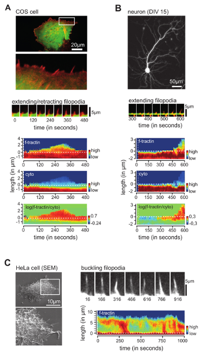
Figure 3: Examples of Filopodia Analyzed by the Software. (A) Overview image (top panel) and time series (middle panel) of COS cells transfected with f-tractin (red) and cytosolic marker (green). Below, plots depicting analysis of filopodial growth dynamics and relative concentration of f-tractin along the filopodium (bottom panels) are shown. (B) Overview image of hippocampal neuron transfected with cytosolic marker (top) and time series of neuron transfected with f-tractin (red) and cytosolic marker (green) (middle panel), as well as plot depicting analysis of dendritic filopodial growth dynamics and relative concentration of f-tractin along the protrusion (bottom panels). (C) SEM image (left panel) and time series of HeLa cells transfected with f-tractin (right panel). Note fluctuations in fluorescence intensity due to filopodial buckling. Scale bars = 20 µm (A, top), 50 µm (B, top), 10 µm (C, top). This figure has been modified from reference 12. Please click here to view a larger version of this figure.
Finally, we aimed to challenge the software by monitoring filopodia in HeLa cells. Filopodia in HeLa cells are long (Figure 3C, left panel) and highly dynamic, often leaving the plane of acquisition. Intriguingly, when focusing on the basal membrane, we observed a sub-fraction of filopodia to undergo helical twisting (Figure 3C, top right panel), whereby parts of the filopodium transiently left the focal plane. Accordingly, kymographs depicting the absolute fluorescence intensity of f-tractin showed wave-like changes in fluorescence intensity through time (Figure 3C, bottom right panel). This behavior is reminiscent of filopodial buckling, a mechanism recently described to be used by filopodia to exert pulling forces 5.
In summary, these experiments provide evidence that the software reliably tracks protein concentration and growth dynamics of filopodial from various origins.
