Lipids are major constituents of membranes, which provide boundaries for cells and enable intracellular compartmentalization1,2,3. Lipids are amphiphilic, with a polar head group and two hydrophobic fatty acid tails; these self-assemble into a bilayer to minimize contact of the hydrophobic chains with water3,4. Various combinations of hydrophilic head groups and hydrophobic tails result in different classes of lipids in biological membranes, such as glycerophospholipids, sphingolipids, and sterols (Figure 1)1,5,6. Glycerophospholipids are primary building blocks of eukaryotic cell membranes composed of glycerophosphate, long-chain fatty acids, and head groups of low-molecular weight7. Lipid nomenclature is based on differences in head groups; examples include phosphatidyl-choline (PC), phosphatidyl-ethanolamine (PE), phosphatidyl-serine (PS), phosphatidyl-glycerol (PG), phosphatidyl-inositol (PI), or the unmodified phosphatidic acid (PA)5,6. As for hydrophobic tails, the length and degree of saturation vary, along with the backbone structure. The possible combinations are numerous, resulting in thousands of lipid species in mammalian cells6. Changes in membrane lipid composition lead to different mechanical and structural membrane properties that impact the activity of both integral membrane proteins and peripheral proteins2,6.
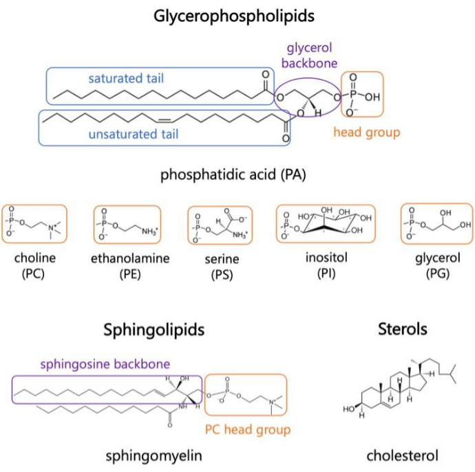
Figure 1. Representative lipid structures. Fatty acid tails are shown in blue boxes, common lipid head groups in orange, and sample backbones in purple. Please click here to view a larger version of this figure.
Lipids are active players in cellular processes, protein activation in signaling cascades, and healthy cell homeostasis8,9. Altered lipid dynamics are the result of infection or can be markers of pathogenesis of disease10,11,12,13,14,15. As barriers for the cell, the study of membrane lipids and their role in permeation of small molecules is of relevance for drug delivery systems and membrane disruption mechanisms16,17. Chemical diversity and different ratios of lipid species across organelles, tissues, and organisms give rise to complex membrane dynamics2. It is therefore important to retain these characteristics in modelling studies of lipid bilayers, especially when the goal of a study is to examine interactions of other biomolecules with the membrane. The lipid species to consider in a model depends on the organism and cellular compartment of interest. For example, PG lipids are important for electron transfer in photosynthetic bateria18, while phosphorylated inositol lipids (PIPs) are major players in plasma membrane (PM) dynamics and signaling cascades in mammalian cells19,20. Inside the cell, the PM, endoplasmic reticulum (ER), Golgi, and mitochondrial membranes contain unique lipid abundances that influence their function. For example, the ER is the hub for lipid biogenesis and transports cholesterol out to the PM and Golgi; it contains a high lipid diversity with an abundance of PC and PE, but low sterol content, which promotes membrane fluidity21,22,23,24. In contrast, the PM incorporates hundreds and even thousands of lipid species depending on the organism25, it contains high levels of sphingolipids and cholesterol that give it a characteristic rigidity compared to other membranes in the cell24. Leaflet asymmetry should be considered for membranes like the PM, which has an outer leaflet rich in sphingomyelin, PC, and cholesterol, and an inner leaflet rich in PE, PI and PS that are important for signaling cascades24. Finally, lipid diversity also prompts the formation of micro-domains that differ in packing and internal order, known as lipid rafts24,26; these exhibit lateral asymmetry, are hypothesized to play important roles in cellular signaling26, and are hard to study due to their transient nature.
Experimental techniques such as fluoroscopy, spectroscopy, and model membrane systems like giant unilamellar vesicles (GUVs) have been used to investigate interactions of biomolecules with membranes. However, the complex and dynamic nature of the components involved is difficult to capture with experimental methods alone. For example, there are limitations on the imaging of transmembrane domains of proteins, the complexity of membranes used in such studies, and the identification of intermediate or transient states during the process of interest27,28,29. Since the advent of molecular simulation of lipid monolayers and bilayers in the 1980s29, lipid-protein systems and their interactions can now be quantified at the molecular level. Molecular dynamics (MD) simulation is a common computational technique that predicts the movement of particles based on their intermolecular forces. An additive interaction potential describes the bonded and non-bonded interactions between particles of the system30. The set of parameters used to model these interactions is termed the simulation forcefield (FF). These parameters are obtained from ab initio computations, semi-empirical, and quantum mechanical calculations, and optimized to reproduced data from X-ray and electron diffraction experiments, NMR, infrared, Raman and neutron spectroscopy, amongst other methods31.
MD simulations can be used to study systems at various levels of resolution32,33,34. Systems that aim to characterize specific biomolecular interactions, hydrogen bonds, and other high-resolution details are studied with all-atom (AA) simulations. In contrast, coarse-grained (CG) simulations lump atoms into larger functional groups to reduce computational cost and examine larger scale dynamics33. Situated in between these two are united-atom (UA) simulations, where hydrogen atoms are combined with their respective heavy atoms to accelerate the computation33,35. MD simulations are a powerful tool for exploration of the dynamics of lipid membranes and their interactions with other molecules and can serve to provide molecular level mechanisms for processes of interest at the membrane interface. Additionally, MD simulations can serve to narrow down experimental targets and predict macromolecular properties of a given system based on microscopic interactions.
In brief, given a set of initial coordinates, velocities, and a set of conditions like constant temperature and pressure, positions and velocities of each particle are calculated through numerical integration of the interaction potential and Newton's Law of motion. This is repeated iteratively, thereby generating a simulation trajectory30. These calculations are performed with an MD engine; among several open-source packages, GROMACS36 is one of the most commonly used engines and the one we describe here. It also includes tools for analysis and constructing initial coordinates of systems to be simulated37. Other MD engines include NAMD38; CHARMM39, and AMBER40, which the user can select at their own discretion based on computational performance of a given system. It is critical to visualize the trajectories during the simulation as well as for analysis and interpretation of the results. A variety of tools are available; here we discuss visual molecular dynamics (VMD) that offers a wide range of features, including three dimensional (3-D) visualization with expansive drawing and coloring methods, volumetric data visualization, building, preparing, and analyzing trajectories of MD simulation systems, and trajectory-movie making with no limits on system size, if the memory is available41,42,43.
The accuracy of predicted dynamics between system components is directly influenced by the FF chosen for the propagation of the trajectory. Empirical FF parametrization efforts are pursued by few research groups. The most established and common FF for MD include CHARMM39, AMBER40, Martini44, OPLS45, and SIRAH46. The all-atom additive CHARMM36 (C36) force field47 is widely used for AA MD of membrane systems as it accurately reproduces experimental structural data. It was originally developed by the CHARMM community, and it is compatible with multiple MD engines like GROMACS and NAMD. Despite improvements across common FFs, there is a continuous effort to improve the parameter sets to allow predictions that closely reproduce experimental observables, driven by interests in particular systems of study48,49.
A challenge when simulating lipid membranes is determining the length of simulation trajectory. This is largely dependent on the metrics to be analyzed and the process that one aims to characterize. Typically, complex lipid mixtures require longer time to reach equilibrium, as more species must have enough time to diffuse on the membrane plane and reach a stable lateral organization. A simulation is said to be at equilibrium when the property of interest has reached a plateau and fluctuates about a constant value. It is common practice to obtain at least 100-200 ns of equilibrated trajectory to carry out appropriate statistical analysis on the properties and interactions of interest. It is common to run membrane-only simulations between 200-500 ns, depending on the complexity of the lipid mixture and research question. Protein-lipid interactions typically require longer simulation times, between 500-2000 ns. Some approaches to accelerate sampling and observable dynamics with membrane systems are: (i) the highly mobile membrane mimetic (HMMM) model, which replaces end carbons of lipids in the membrane with organic solvent to accelerate sampling50; and (ii) hydrogen mass repartitioning (HMR), which combines a fraction of the masses of heavy atoms within a system with those of hydrogen atoms to allow the use of a larger simulation timestep51.
The following protocol discusses a beginner-friendly approach to build, run, and analyze realistic membrane models using AA MD. Given the nature of MD simulations, multiple trajectories must be run to account for reproducibility and proper statistical analysis of the results. It is current practice to run at minimum three replicas per system of interest. Once the lipid species have been selected for the organism and process of interest, basic steps to build, run, and analyze a simulation trajectory of a membrane-only system are outlined and summarized in Figure 2.
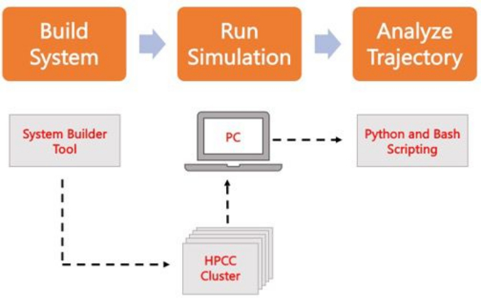
Figure 2. Schematic to run MD simulations. Orange boxes correspond to the three main steps described in the protocol. Underneath is the workflow of the simulation process. During system setup, the system containing the initial coordinates of a solvated membrane system is built with a system input generator like CHARMM-GUI Membrane Builder. After transferring the input files to a high-performance computing cluster, the simulation trajectory is propagated using an MD engine, such as GROMACS. Trajectory analysis can be done on the computer cluster or a local working station along with visualization. Analysis is then carried out, using either packages with built-in analysis code such as GROMACS and VMD, or by using Bash scripts or various Python libraries. Please click here to view a larger version of this figure.
To illustrate the use of the protocol and the results that can be obtained, a comparison study for membrane models for the endoplasmic reticulum (ER) is discussed. The two models in this study were (i) the PI model, which contains the top four lipid species found in the ER, and (ii) the PI-PS model, which added the anionic phosphatidylserine (PS) lipid species. These models were later used in a study of a viral protein and how it interacts with the membrane, the interest on PS has been cited as important for the permeabilization activity of the viral protein23. To incorporate variety in lipid tail structures, the membrane compositions were set as DOPC:DPPE:CHOL:POPI (56:22:10:12 mol%) and DOPC:DPPE:CHOL:POPI:DOPS (55:21:11:9:4 mol%).
The membranes were generated with CHARMM-GUI Membrane Builder. To accommodate the 4 different lipid species and later the protein, the symmetric membranes were set to contain 600 lipids/leaflet. The settings recommended in the protocol were used, with a temperature of 303 K. To ensure independent replicas, the building process was repeated three times for each membrane model, resulting in a different random mixture of lipids each time. After building the systems, the input files were moved to the UB center for computational research (CCR) high-performance computing cluster55 to run MD simulations using GROMACS version 2020.5. After the 6-step relaxation protocol was completed, benchmarking was performed on only one system per model (Figure 3) since the number of atoms are similar across all replicas. The 75% of the maximum performance was ~78 ns/day, hence, at most 6 nodes were requested on the cluster for the production runs. Each replica was run for up to 500 ns by setting nstep = 25 x 107 in the *.mdp file and submitting extensions to the cluster as needed based on the benchmarks.
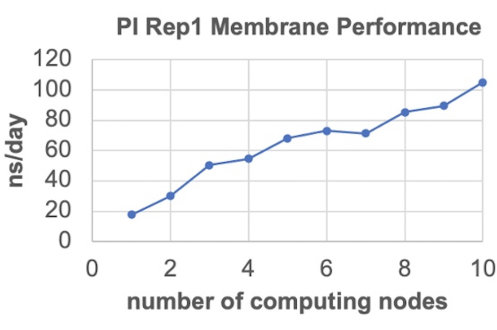
Figure 3. Sample benchmark runs. Used to determine performance of the PI Model (315,000 atoms). Please click here to view a larger version of this figure.
The area-per-lipid (APL) for each replica is shown in Figure 4. This was computed from the XY dimensions of the simulation box stored in the *edr simulation output file from GROMACS using the energy built-in program. Then, the total surface area was divided by the number of total lipids per leaflet to provide an estimate of the APL in each model. For all systems, equilibration was determined as the point where the APL reaches a plateau and fluctuates about a constant value. In all these systems, equilibrium is reached within the first 100 ns of trajectory (see Figure 4). Based on this metric, trajectories of 500 ns were deemed enough for these systems. All other analysis on these bilayers was carried out over the last 400 ns of trajectory, known as the equilibrated or production phase. To determine the uncertainty in each computed value, block-averaging every 10-20 ns is recommended. From the APL analysis, the PI-PS membrane model has, on average, a 0.7 Å2 larger surface area than the PI model.
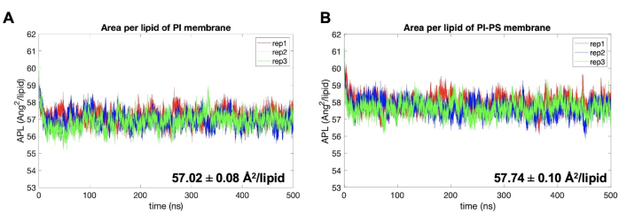
Figure 4. Area-per-lipid examples. (A) PI and (B) PI-PS models. Replicate 1, replicate 2, and replicate 3 for each model are shown in red, blue, and green. Equilibration for all systems occur within first 100 ns. Uncertainty is reported as the standard error of the mean (SEM). Please click here to view a larger version of this figure.
In addition, two simple analyses on membrane structure are presented. Figure 5 shows the membrane thickness, estimated by the distance between the center of mass (COM) of the phosphate atoms of phospholipids in the top and bottom leaflets. This was computed using the distance program in GROMACS, which requires an index file that lists two atom groups, one for the phosphate groups in the top leaflet and another group for those in the bottom leaflet. The results show a statistical difference between the thicknesses of the two membrane models, illustrating an inverse relation between APL and membrane thickness. Finally, Figure 6 shows the deuterium order parameters of each lipid species, a measure that quantifies the order of lipid tails within the bilayer hydrophobic core56. Fatty acid tails are classified as sn1, the one attached to the terminal oxygen of the glycerol backbone, and sn2, attached to the central oxygen of the glycerol group. The results show there is little to no difference between the order of lipid tails between the models, except for DPPE that shows a slight increase in order for the sn1 tail in the PI model.
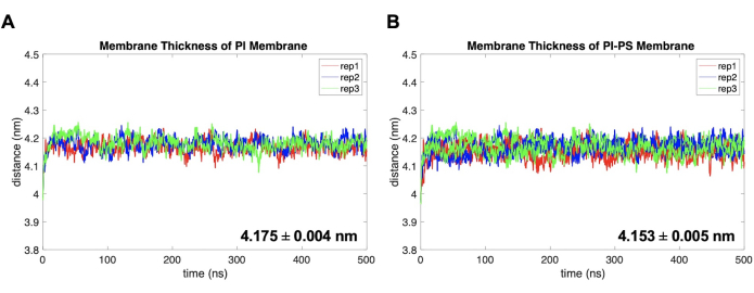
Figure 5. Membrane thickness examples. (A) PI and (B) PI-PS models. Replicate 1, replicate 2, and replicate 3 for each model are shown in red, blue, and green. Uncertainty is reported as the standard error of the mean (SEM). Please click here to view a larger version of this figure.
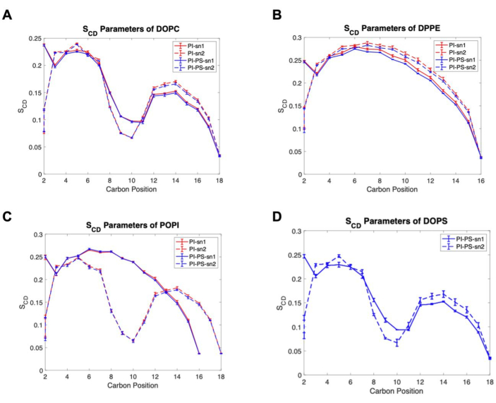
Figure 6. Deuterium order parameters examples. (A) DOPC, (B) DPPE, (C) POPI, and (D) DOPS lipid species. Solid lines for sn1, dashed lines for sn2, PI model in red, and PI-PS model in blue. Uncertainty is reported as the standard error of the mean (SEM). Please click here to view a larger version of this figure.
Complex membrane models can be used to study the relevance of specific lipid species and how these modulate interactions of biomolecules with the membrane. Sample studies from the lab show: (1) membrane composition modulates the interactions of proteins19, and (2) lipid tail saturation and membrane surface charge impact permeation and lateral organization of small molecules17,57. Using the protocol described above and similar analysis as that presented in previous paragraphs, the work by Li et al. provides insights from experiment and simulation on the interplay between D112, a potential photodynamic therapy agent, and different lipid mixtures17. A bilayer with PC and PS lipids was examined in an experiment to characterize D112 partitioning in the bilayer. We carried out simulations of different rations of PC and PS lipids, with varying fatty acid tail lengths and saturation, i.e., number of double bonds, to determine the effect of surface charge and hydrophobic environment on D112-membrane interaction. While electrostatic interactions drive initial binding of D112 to anionic PS lipids, hydrophobic interactions pull the molecule into the membrane core via two possible mechanisms (see Figure 7A-B). Inside the membrane, D112 preferentially localizes to PC-rich domains, either as a monomer or dimer.
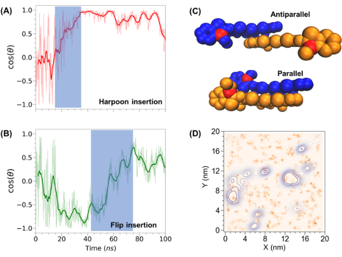
Figure 7. Additional sample system following the presented protocol. Simulations of D112 with model membranes identifying two insertion mechanisms (A) harpoon and (B) flip; (C) orientation of D112 dimers; and (D) lateral distribution of D112 molecules (blue contour maps) on a membrane model with respect to charged lipids (orange clusters). Full study can be found in 17. Please click here to view a larger version of this figure.
