JoVE Science Education
Biomedical Engineering
É necessária uma assinatura da JoVE para visualizar este conteúdo.  Faça login ou comece sua avaliação gratuita.
JoVE Science Education Biomedical Engineering
Computational Fluid Dynamics Simulations of Blood Flow in a Cerebral Aneurysm
  • 00:07Visão Geral
  • 01:20Principles of Computational Fluid Dynamics
  • 03:15Generating Vessel Centerlines
  • 04:24Remapping 4D Flow MRI and Determining the Boundary Conditions
  • 08:09CFD Simulations
  • 10:22Resultados
  • 11:17Applications
  • 12:17Summary

Simulations numériques de la dynamique des fluides du flux sanguin lors d'un anévrisme cérébral

English

COMPARTILHAR

Visão Geral

Source: Joseph C. Muskat, Vitaliy L. Rayz, et Craig J. Goergen, Weldon School of Biomedical Engineering, Purdue University, West Lafayette, Indiana

L’objectif de cette vidéo est de décrire les progrès récents des simulations de dynamique des fluides computationnels (CFD) basées sur la vascularisation spécifique au patient ou à l’animal. En l’espèce, des segmentations de navires en question ont été créées et, à l’aide d’une combinaison d’outils open source et commerciaux, une solution numérique à haute résolution a été déterminée dans un modèle d’écoulement. De nombreuses études ont démontré que les conditions hémodynamiques dans la vascularisation affectent le développement et la progression de l’athérosclérose, des anévrismes, et d’autres maladies périphériques d’artère ; en même temps, les mesures directes de la pression intraluminale, du stress de cisaillement de mur (WSS), et du temps de résidence de particule (PRT) sont difficiles à acquérir in vivo.

Le CFD permet d’évaluer ces variables de manière non invasive. En outre, le CFD est utilisé pour simuler des techniques chirurgicales, ce qui permet aux médecins de mieux faire preuve de prévoyance en ce qui concerne les conditions de débit postopératoire. Deux méthodes d’imagerie par résonance magnétique (IRM), d’angiographie par résonance magnétique (MRA) avec un temps de vol (TOF-MRA) ou un MRA amélioré par contraste (CE-MRA) et un contraste de phase (PC-MRI), nous permettent d’obtenir des géométries de navires et des champs de vitesse 3D résolus dans le temps. Respectivement. TOF-MRA est basé sur la suppression du signal à partir de tissu statique par des impulsions RF répétées qui sont appliquées sur le volume image. Un signal est obtenu à partir de spins insaturés se déplaçant dans le volume avec le sang qui coule. CE-MRA est une meilleure technique pour l’imagerie des navires avec des flux de recirculation complexes, car il utilise un agent de contraste, comme le gadolinium, pour augmenter le signal.

Séparément, PC-MRI utilise des gradients bipolaires pour générer des décalages de phase qui sont proportionnels à la vitesse d’un fluide, fournissant ainsi des distributions de vitesse résolues dans le temps. Tandis que PC-MRI est capable de fournir des vitesses de flux sanguin, la précision de cette méthode est affectée par la résolution spatiotemporal limitée et la gamme dynamique de vitesse. CFD fournit une résolution supérieure et peut évaluer la gamme de vitesses des jets à grande vitesse à la recirculation lente des tourbillons observés dans les vaisseaux sanguins malades. Ainsi, même si la fiabilité du CFD dépend des hypothèses de modélisation, elle ouvre la possibilité d’une représentation complète et de haute qualité des champs d’écoulement spécifiques aux patients, qui peuvent guider le diagnostic et le traitement.

Princípios

Procedimento

Un précurseur du tutoriel est la création d’un modèle de vascularisation spécifique au patient. Dans cette démonstration, les outils Materialise Mimics, 3D Systems Geomagic Design X et Altair HyperMesh ont été utilisés pour générer un maillage de volume tétraèdre à partir de données MRA. 1. Générer des lignes maîtresses de navire pour le modèle Ouvrez le vmtk-lanceur python GUI. Dans le PypePad, tapez : vmtkcenterlines -ifile [fichier STL enregistré sur le bure…

Resultados

In this demonstration, a subject-specific model of a cerebral aneurysm was generated and the CFD was used to simulate the flow field. By providing detailed flow features and quantifying hemodynamics forces not obtainable from imaging data, CFD can be used to augment lower resolution 4D Flow MRI data.  Figure 1 shows how CFD gives a more complete description of the flow in the near-wall, re-circulating regions.

Figure 1
Figure 1: A) Visualization of 4D Flow MRI data within the vessel geometry. B) Visualization of CFD simulation results. In general, CFD streamlines give fuller understanding of blood flow patterns within this cerebral aneurysm.

Figure 1 shows that CFD results are in agreement with in vivo 4D Flow MRI. Figure 1 (A) shows the complex, recirculating flow patterns within the aneurysmal region, the balloon-like dilatation of the artery, which were detected with 4D Flow MRI. However, regions of stagnant flow in the top and bottom sections of the lesion are not filled with streamlines. This is because the signal to noise ratio in these regions is low. CFD-simulated flow, shown in Figure 1 (B), provides a higher resolution velocity field, particularly near the vessel walls. Thus, CFD models are capable of providing higher accuracy estimates of clinically-relevant, flow-derived metrics, such as pressure, WSS, and PRT, which can be used to predict aneurysmal disease progression.

Additionally, CFD simulations can be used to model postoperative flow conditions that would result from alternative treatment options. For example, Figure 2 (A) and (B) compare flow through the same vessel with different inflow rates. By prescribing varied boundary conditions, such as simulating vessel occlusion with no flow, the flow after a variety of surgical treatments is shown.

Figure 2
Figure 2: A) Simulation for surgical clipping of the right anterior cerebral artery (ACA). B) Simulation for surgical clipping of the left ACA. For simplicity, this figure maintains the preoperative inflow rate at the non-modified inlet; in reality, the flow rate would increase in the open vessel to compensate. C) Normal blood flow rates prescribe the inlet conditions for this model. Patient data from 4D Flow MRI provide inlet conditions for realistic visualization of flow patterns.

The ability to simulate postoperative flow fields resulting from various surgical treatments is an important advantage of CFD models. By applying realistic, patient-specific geometries and inflow data, different treatment scenarios can be demonstrated to provide physicians with information on the effect of a planned procedure on flow patterns. For example, Figure 2 (A) and (B) show recirculating flows that would occur if one or the other proximal artery is clipped. Treatments such as vessel clipping or deploying a flow diverter can be simulated, allowing physicians and patients to decide what will work best in each specific case.

Applications and Summary

The framework described here can be used to perform patient-specific CFD simulations. A high-resolution mesh is used to interpolate low-resolution 4D Flow MRI data; this isolates the flow data and minimizes error associated with noise external to the vessel wall. By using patient-based boundary conditions for the inlet and outlet flows, the simulation is capable of matching the hemodynamic conditions imaged with MRI.

Novel methods for PC-MRI are capable of showing larger, dynamic ranges of velocities. However, this is severely limited by patient scan time. Often, patient data are acquired at lower resolutions to reduce the time spent within the scanner. Unfortunately, this can result either in aliased data or signal drop-off, a problem exacerbated when the velocity encoding gradient (VENC) is set too high. This can miss slow and recirculating flow data. Pairing patient-specific flow and geometry with CFD provides an effective method for capturing high-resolution blood flow dynamics.

What makes patient-based modeling inherently useful is its ability to provide detailed information without the need to generalize across patients, diseases, or treatments that typically possess very different characteristics. Simulations allow for physicians and engineers to model alternative treatment scenarios before performing an actual procedure. Simulating blood flow dynamics can be used to model flow diverting stents, artery bypass grafting, and catheter-based contrast injection, among other applications. While clinicians and patients wish for the best outcome, CFD provides a method for looking at post-operative flow, which provides better foresight. Apart from depicting flow after introducing a device or treatment, CFD allows for estimations of shear stresses at the wall. This, paired with knowledge that low WSS often correlates to arterial disease progression, allows for prediction or probability modeling. Using computational tools to identify precursors to aneurysm growth, clot formation, or hemorrhage opens the possibility of identifying at-risk patients earlier. In summary, the combination of patient-specific image data with CFD simulations is a powerful tool for disease assessment and surgical prediction.

ACKNOWLEDGEMENTS

The authors would like to thank Dr. Susanne Schnell and Michael Markl at Northwestern University for providing us with the 4D patient data used in our figures.

Transcrição

Computational fluid dynamic simulations are used to analyze blood flow in patient vasculature to guide diagnostics and treatment. Computational fluid dynamics, or CFD, uses numerical analysis methods to model fluid flow and simulate realistic conditions for many different flow scenarios, such as the fluid flow around a high-speed airplane, through complex piping networks, and within our cardiovascular system.

In medical application, various imaging techniques are used to obtain blood vessel geometries. Then CFD simulations are performed, which are used to predict disease progression and model treatment scenarios for vasculature dysfunctions, including coronary heart disease, arteriovenous malformations, and aneurysms.

This video will illustrate the principles of CFD, demonstrate how the geometries of blood vessels are used to model high resolution hemodynamics, and discuss some applications of CFD.

First, let’s understand cardiovascular dynamics and the principles of CFD.

Cardiovascular hemodynamics describes the dynamics of blood flow in the heart, including through the left and right ventricles and atria, and blood flow in the vessels from the heart to the rest of the body. Complex vascular networks can be visualized using magnetic resonance angiography and velocimetry or X-ray fluoroscopy. These methods outline the geometry of the patient’s blood vessels and define flow boundary conditions.

Once this is acquired, the blood velocity data are segmented into voxels, which are units of graphical information defining a 3D space, and the phase shift is obtained at each voxel. These depend on the gyromagnetic ratio, the main magnetic field, the applied gradient field, and the position of the spin. This in turn depends on the initial position of the spin, the spin velocity, and the spin acceleration. Tau is the time that defines the fourth dimension.

These parameters are defined by the MRI and input into CFD simulations. The 3D flow velocity is determined by numerically solving the Navier-Stokes or NS equations. The NS equations are the governing equations of fluid motion solved to determine velocity and pressure distributions. They take into account the density, velocity, pressure, and dynamic viscosity of the flow.

We will now see how these principles of fluid dynamics are applied to real blood vessel geometries to produce high resolution CFD simulations.

Before starting, create a patient-specific vasculature model from MRA data. This can be done using open source software for image segmentation.

For this demonstration, a tetrahedral volume mesh was generated. Now open the vmtk launcher Python GUI. In the PypePad, enter in the necessary file name. This bare bones command will pull the input STL file from the desktop. Select Run, Run all to load the data into the program. A new window will open that displays instructions and a rendering of the input model.

Rotate the model and place the cursor on each inlet location. Press the space bar to place a seed on one inlet. Repeat this for all inlets. Then press Q to continue. Now repeat the same placement of seeds for all outlets. Press Q again and let the program run. The centerline file will be generated and saved to the desktop.

We are now ready to use the open source visualization tool ParaView to separate the voxels containing flow data from stationary tissue. Locate the following files: the patient-specific volume mesh, Centerline files, and the EnSight.case files and click OK to load the data onto the interface. Navigate to the Properties table and select Apply to load and read all the information. Then highlight the volumetric mesh in the pipeline browser.

In the Properties table, change the opacity value to between 0.2 and 0.5. The centerlines and geometric rendering should now be visible. Next, go to the top menu and select Filters, Alphabetical, Resample With Dataset, and set the source as the volume mesh and the input as the EnSight.case file. Click OK to continue, and apply the filter in the Properties table. Then, highlight the new Resample With Dataset and reduce the opacity.

From the top menu, change the centerlines from Surface to Points. To determine the boundary conditions, go to the right side of the interface and select the Split Horizontal Create View tool. Choose the SpreadSheet View option. From the Showing dropdown box, select the Centerline file and cycle through the files, selecting various points to identify a location within each inlet and outlet. Now use the SpreadSheet View to calculate the normal vector between two points.

After finding the vector, activate the ResampleWithDataset and select Filters, Alphabetical, Slice. Make sure the Slice filter appears, then go to the Properties table and set the plane origin as the same X, Y, Z point location for one of the two points used to calculate the normal vector. Use this to fill out the normal values, then select Apply. Activate the newly created Slice filter and select Filters, Alphabetical, Surface Flow. Click Apply, then activate the new Surface Flow item, followed by Filters, Alphabetical, Group Time Steps, Apply.

In SpreadSheet View, open the GroupTimeSteps data and use Export Spreadsheet or copy-paste to export this data to Microsoft Excel. Within ParaView, determine the Time Steps and the Time Step size by cycling through Time. For the simulation, we want the cardiac cycle to start at time equals zero. Therefore, generate the adequate time scale. Then activate the Slice filter and select Filters, Alphabetical, Integrate Variables.

From the pop-up, change Attribute to display Cell Data. This provide you with the cross-sectional area of the inlet slice. To make the flow data compatible with ANSYS Fluent, determine the time scale with units of seconds and the inlet velocity with units of meters per second.

The first line must contain a data name, a number of columns, number of rows, and a binary trigger for repeatability. The next line contains the names for each of the data columns. The flow velocities, not rates, are set underneath the respective column header. In order to simulate multiple cardiac cycles smoothly, the initial and final velocity values should be equivalent.

Chose File, Read, Case, and open the volume mesh .cas file that was used previously. Check the box for Display Mesh After Reading to show the mesh once imported. Select Scale and apply the necessary unit conversion to ensure correct physical size of the model. Select Materials Create/Edit, and input material properties for blood.

Now, select the Console command window and input file/. Use read-transient-table to import the transient flow waveforms located in the same location as the volume mesh .cas file. Use the waveforms obtained from the 4D flow MRI measurements to set the inlet boundary conditions. Then use a weighted ratio of inlet to outlet to set the outlet boundary conditions.

Set the numerical schemes used for pressure velocity coupling and discretization of the Navier-Stokes equations. Then, within Solution Initialization, set all the Initial Values to zero. Under Calculation Activities, designate a solution folder to save the results and specify the frequency with Autosave, Every Time Steps. Under Run Calculation, set up the Time Step Size from the Excel boundary conditions data. It is often preferable to select a smaller Time Step and allow Fluent to interpolate. Repeat for at least three cardiac cycles.

Finally, set the Max Iterations between 300 and 500. The software will automatically stop the iterations at each Time Step once the convergence occurs. After the simulation has been fully set up, go back to Initialization, Initialize. Return to Run Calculation and select Calculate to run the solver. The solution data can now be visualized in either ANSYS CFD-Post or ParaView software.

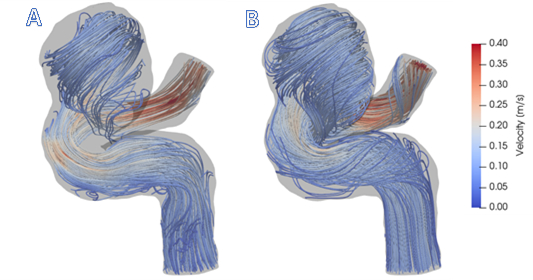
We will now examine some representative data. Here is an example of a cerebral aneurysm. From 4D flow MRI data, complex recirculating flow patterns within the aneurysmal region were detected. However, the resolution is limited in the regions of stagnant flow observed in the top and bottom section of the lesion. After running CFD simulations, higher resolution of the velocity field was obtained, particularly near the vessel walls.

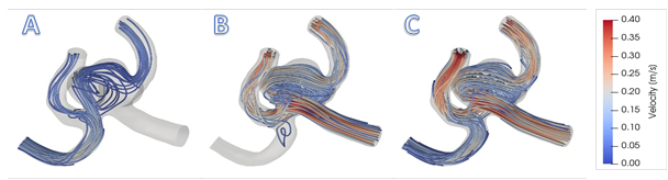
CFD can also be used to compare different flow conditions in the same vessel. For instance, simulations of a surgical clipping of the right and left anterior cerebral artery help visualize the effects of the procedure on flow dynamics.

Computational fluid dynamic simulations of blood flow are useful tools used in various biomedical applications.

For example, hemodynamic conditions within the vasculature affect development and progression of arterial diseases, including atherosclerosis and aneurysms. Since direct measurements are difficult to acquire in vivo, CFD is a standard research tool that is used to model blood flow dynamics. It can provide physicians guidance for diagnostics, as well as different treatment scenarios.

On top of vascular modeling, CFD simulations serve to simulate airflow based on nasal airway models. It is particularly useful to design protocols to deliver, in an adequate and controlled manner, pharmaceutical aerosols to targeted olfactory regions that interact directly with the brain.

You’ve just watched JoVE’s introduction to computational fluid dynamics to simulate blood flow. You should now understand how high resolution blood flow dynamics can be modeled based on three-dimensional vessel geometries. Thanks for watching!

Tags

Cite This
JoVE Science Education Database. JoVE Science Education. Computational Fluid Dynamics Simulations of Blood Flow in a Cerebral Aneurysm. JoVE, Cambridge, MA, (2023).