Fuente: Dominique R. Bollino1, Eric A. Legenzov2, Tonya J. Webb1
1 Departamento de Microbiología e Inmunología, Facultad de Medicina de la Universidad de Maryland y el Centro Integral del Cáncer Marlene y Stewart Greenebaum, Baltimore, Maryland 21201
2 Centro de Ingeniería y Tecnología Biomédica, Facultad de Medicina de la Universidad de Maryland, Baltimore, Maryland 21201
La microscopía de fluorescencia confocal es una técnica de imagen que permite una mayor resolución óptica en comparación con la microscopía de epifluorescencia convencional de “campo ancho”. Los microscopios confocales son capaces de lograr una resolución óptica x-y mejorada a través del “escaneo láser”, normalmente un conjunto de espejos controlados por voltaje (galvanómetro o espejos “galvo”) que dirigen la iluminación láser a cada píxel de la muestra a la vez. Lo que es más importante, los microscopios confocales logran una resolución z-axial superior mediante el uso de un agujero para eliminar la luz de foco procedente de lugares que no están en el plano z que se está escaneando, lo que permite al detector recopilar datos de un plano z especificado. Debido a la alta resolución z alcanzable en la microscopía confocal, es posible recopilar imágenes de una serie de planos z (también llamados z-stack) y construir una imagen 3D a través de software.
Antes de discutir el mecanismo de un microscopio confocal, es importante considerar cómo interactúa una muestra con la luz. La luz se compone de fotones, paquetes de energía electromagnética. Un fotón que afecta a una muestra biológica puede interactuar con las moléculas que componen la muestra de una de cuatro maneras: 1) el fotón no interactúa y pasa a través de la muestra; 2) el fotón se refleja / dispersa; 3) el fotón es absorbido por una molécula y la energía absorbida se libera como calor a través de procesos conocidos colectivamente como descomposición no radiativa; y 4) el fotón se absorbe y la energía se emite rápidamente como un fotón secundario a través del proceso conocido como fluorescencia. Una molécula cuya estructura permite la emisión de fluorescencia se llama fluoróforo. La mayoría de las muestras biológicas contienen fluoróforos endógenos insignificantes; por lo tanto, los fluoróforos exógenos deben utilizarse para resaltar las características de interés en la muestra. Durante la microscopía de fluorescencia, la muestra se ilumina con luz de la longitud de onda adecuada para la absorción por el fluoróforo. Al absorber un fotón, se dice que un fluoróforo está “emocionado” y el proceso de absorción se conoce como “excitación”. Cuando un fluoróforo renuncia a la energía en forma de fotón, el proceso se conoce como “emisión”, y el fotón emitido se llama fluorescencia.
El haz de luz utilizado para excitar un fluoróforo está enfocado por la lente objetivo de un microscopio y converge en un “punto focal” donde se centra al máximo. Más allá del punto focal, la luz vuelve a divergir. Las vigas de entrada y salida se pueden visualizar como un par de conos que se tocan en el punto focal (consulte la figura 1, panel izquierdo). El fenómeno de la difracción impone un límite a la tensión con la que se puede enfocar un haz de luz : el haz en realidad se centra en un punto de tamaño finito. Dos factores determinan el tamaño del punto focal: 1) la longitud de onda de la luz, y 2) la capacidad de recolección de luz de la lente objetivo, que se caracteriza por su apertura numérica (NA). El “punto” focal se extiende no sólo en el plano x-y, sino también en la dirección z, y en realidad es un volumen focal. Las dimensiones de este volumen focal definen la resolución máxima alcanzable por imágenes ópticas. Aunque el número de fotones es mayor dentro del volumen focal, las trayectorias de luz cónicas por encima y por debajo del foco también contienen una densidad más baja de fotones. Cualquier fluoróforo en el camino de luz puede ser excitado. En la microscopía de epifluorescencia convencional (de campo ancho), la emisión de fluoróforos por encima y por debajo del plano focal contribuye a la fluorescencia fuera de foco (un “fondo de superficie”), que reduce la resolución y el contraste de la imagen, como se demuestra en la Figura 1, con el cubo rojo que representa la emisión de fluoróforo por encima del plano focal (estrella roja) que resulta en fluorescencia desenfocada (arriba a la derecha). Este problema se mejora en microscopía confocal, debido a la utilización de un agujero. (Figura 2, abajo a la derecha). Como se muestra en la Figura 3, el agujero permite que las emisiones procedentes del lugar focal lleguen al detector (izquierda), al tiempo que bloquea la fluorescencia desenfocada (derecha) de llegar al detector, mejorando así tanto la resolución como el contraste.
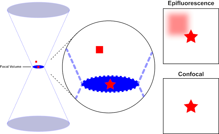
Figura 1. Resolución óptica de epifluorescencia frente a microscopía confocal. Haga clic aquí para ver una versión más grande de esta figura.
El haz de luz utilizado para excitar un fluoróforo está enfocado por la lente objetivo de un microscopio y converge en un volumen focal y luego diverge (izquierda). La estrella roja representa el plano focal de una muestra que se está siendo imagenda mientras que el cuadrado rojo representa la emisión de fluoróforo por encima del plano focal. Al capturar una imagen de esta muestra utilizando un microscopio epifluorescente, la emisión desde el cuadrado rojo fuera de foco será visible y contribuirá a un “fondo brumoso” (arriba a la derecha). Los microscopios confocales tienen un agujero que impide la detección de la luz emitida fuera del plano focal, eliminando el “fondo brumoso” (abajo a la derecha).

Figura 2. Efecto agujero en microscopía confocal. Haga clic aquí para ver una versión más grande de esta figura.
Aunque la intensidad más alta de la luz de excitación se encuentra en el punto focal de la lente (izquierda, óvalo rojo), otras partes de la muestra que no están en el punto focal (derecha, estrella roja) obtendrán luz y flúor. Para evitar que la luz emitida por estas regiones fuera de foco llegue al detector, hay una pantalla con un agujero delante del detector. Sólo la luz de enfoque (izquierda) que emite desde el plano focal es capaz de viajar a través del agujero y llegar al detector. La luz desenfocada (derecha) está bloqueada con el agujero y no llega al detector.
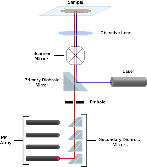
Figura 3. Componentes principales de un microscopio de escaneo láser confocal. Haga clic aquí para ver una versión más grande de esta figura.
En aras de la simplicidad, la descripción mecanicista de un microscopio confocal se limitará a la de la Nikon Eclipse Ti A1R. Aunque puede haber pequeñas diferencias técnicas entre diferentes microscopios confocales, el A1R sirve bien como un buen modelo para describir la función del microscopio confocal. El haz de luz de excitación, producido por una serie de láseres de diodos, se refleja en el espejo dicrosico primario en el objetivo, que centra la luz en la muestra que se está realizando. El espejo dicoico primario refleja selectivamente la luz de excitación mientras permite que la luz en otras longitudes de onda pase a través. A continuación, la luz se encuentra con los espejos de escaneo que barren el haz de luz a través de la muestra de una manera x-y, iluminando un solo píxel (x,y) a la vez. La fluorescencia emitida por los fluoróforos en el píxel iluminado es recogida por la lente objetivo y pasa a través del espejo dicrromico primario para llegar a una serie de tubos fotomultiplicadores (PMP). Los espejos dicoicos secundarios dirigen la luz de emisión a la PMT apropiada. La luz de excitación dispersa por la muestra de nuevo en el objetivo se refleja en el espejo dicroro primario hacia la muestra, y así se impide que entre en la detección camino de luz y alcanzando los PMT (véase el cuadro 3). Esto permite cuantificar la fluorescencia relativamente débil sin contaminación por la luz dispersa del haz de luz de excitación, que suele ser órdenes de magnitud más intensas que la fluorescencia. Debido a que el agujero bloquea la luz desde fuera del volumen focal, la luz que llega al detector proviene de un plano zestrecho y seleccionado. Por lo tanto, las imágenes se pueden recoger de una serie de planos zadyacentes; esta serie de imágenes se conoce a menudo como una ‘z-pila’. Mediante el uso del software adecuado, se puede procesar una z-stack para generar una imagen 3D de la muestra. Una ventaja particular de la microscopía confocal es la capacidad de distinguir la localización subcelular de la tinción. Por ejemplo, la diferenciación entre la tinción de membrana de la tinción intracelular, que es muy difícil con la microscopía de epifluorescencia convencional (1, 2, 3).
La preparación de muestras es una faceta importante de las imágenes confocales. Una fuerza de las técnicas de microscopía óptica es la flexibilidad para crear imágenes de células vivas o fijas. Al intentar producir imágenes 3D, debido al número de imágenes que se deben adquirir para una pila z, la dificultad de mantener la salud celular, y el movimiento de las células vivas y sus orgánulos, el uso de células fijas es típico. El procedimiento de fijación y tinción de células para fluorescencia confocal es similar al utilizado convencionalmente en inmunofluorescencia. Después del cultivo en diapositivas de cámara o en cubreobjetos, las células se fijan usando paraformaldehyde para preservar la morfología celular. La unión de anticuerpos no específica se bloquea mediante albúmina de suero bovino, leche o suero normal. Con el fin de mantener la especificidad de los anticuerpos secundarios, la solución utilizada no debe proceder de la misma especie en la que se generaron los anticuerpos primarios. Las células se incuban con anticuerpos primarios que unen el antígeno de interés. Al etiquetar varios objetivos celulares, los anticuerpos primarios deben derivarse cada uno de una especie diferente. Los anticuerpos que etiqueten un antígeno están unidos por anticuerpos secundarios conjugados con fluoróforos. Se deben seleccionar anticuerpos secundarios conjugados con fluoróforos para que sean compatibles con las longitudes de onda de excitación láser disponibles en el microscopio confocal. Al visualizar múltiples antígenos, los espectros de excitación/emisión de los fluoróforos deben diferir lo suficiente para que sus señales puedan ser discriminadas por análisis microscópicos. La muestra manchada se monta en un portaobjetos para obtener imágenes. Se utiliza un medio de montaje para prevenir el fotoblanqueo y la deshidratación de muestras. Si lo desea, se puede utilizar un medio de montaje que contenga una contramancha nuclear (por ejemplo, DAPI o Hoechst) (4).
En el siguiente protocolo, los fibroblastos de ratón transinfectados para expresar CD1d (LCD1) se tiñieron con anticuerpos que reconocieron CD1d y CD107a (LAMP-1). CD1d es un importante complejo de histocompatibilidad 1 (MHC 1) -como receptor presente en la superficie del antígeno que presenta antígenos lipídicos. LAMP-1 (proteína de membrana asociada a la islosomal-1) es una proteína transmembrana presente principalmente en las membranas lisosomal. Para una correcta presentación del antígeno, CD1d se trafica a través del compartimento lisosomal de pH bajo, por lo que LAMP-1 se utiliza como marcador del compartimento lisosomal para este protocolo. Al sondear las células LCD1 con anti-CD1d y anti- LAMP-1 que se produjeron en diferentes especies, se pueden utilizar anticuerpos secundarios con fluoróforos únicos para determinar la localización de cada proteína en la célula y si CD1d está presente en el LAMP-1 positivo compartimentos lisosomal.
In this experiment, mouse fibroblasts expressing the surface glycoprotein gene CD1d were fixed, immunostained and imaged on a confocal microscope. A representative image obtained using the above protocol is shown in Figure 4. In the top panel of A, single-channel images showing the staining pattern of each individual target are presented. These images comprise a single section (slice) of the z-stack captured. The right panel shows DAPI staining of nuclei of the cells. The center panels show CD1d stained in red and LAMP-1, a lysosomal marker, stained in green. The left panel is a composite image where the three different channels are merged. The appearance of yellow results from overlap of the red and green channels, and indicates an area where CD1d and LAMP-1 are co-localized. The results of the staining confirm that CD1d is localized in the LAMP-1+ endosomal compartments. There are also areas where only one color is present, which indicates the presence of CD1d or LAMP-1 without co-localization. The bottom panel of A shows a 3D rendering of the cells constructed from images captured in the z-stack.
Panel B shows a slice out of the z-stack at 100x magnification demonstrating the expression patterns of these two proteins in greater detail. The pink outlined box on the right side of the image displays the cross section of the x-coordinate designated by the pink line in the image, which represents the side view at the pink line. Similarly, the blue outlined box on the bottom of the image shows the cross section of the y-coordinate designated by the blue line in the image, which represents the front view at the blue line. The 3D rendering of the z-stack image enables users to view the image in 3D, visualizing all the x, y and z planes.
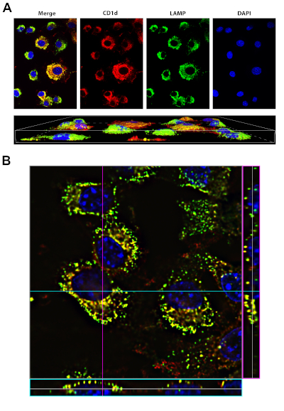
Figure 4: Staining of CD1d and LAMP1. Please click here to view a larger version of this figure.
A, top panel: LCD1 cells were fixed, permeabilized and stained with antibodies to CD1d (red) and LAMP-1 (green, a marker of the lysosomal compartment). DAPI (blue, was used to visualize the nucleus). The merge (left panel) shows that CD1d is localized in the LAMP-1 positive late endosomal/lysosomal compartment (yellow).
A, bottom panel: 3D rendering of the same cells in top panel. Images were acquired using a 40x oil-immersion objective on the Nikon Eclipse Ti, using the NIS Elements Advanced Research software.
B: 100x image of LCD1d cells stained as in A, with stack information for a particular y-coordinate (denoted by the blue line) on the bottom of the image (blue box). The stack information for a particular x-coordinate (denoted by the pink line) is shown on the right side of the image (pink box).
Confocal fluorescent staining is a relatively simple procedure that results in extremely high-quality images of specimens that are prepared in a similar way as for conventional fluorescence microscopy. In brief, samples are fixed, permeabilized, then blocked. Primary antibodies against a protein or proteins of interest are allowed to bind, then fluorophore-conjugated secondary antibodies are used to visualize the staining. Confocal fluorescence microscopy has applications in many areas of research. For example, by staining for markers of sub-cellular organelles along with a protein of interest, confocal microscopy can be used to determine the subcellular locations of diverse proteins. Compared to conventional fluorescence microscopy, confocal imaging can more effectively distinguish between cell surface and intracellular location of a protein. In addition, confocal imaging can also be used to determine whether two proteins co-localize within the cell. Although not outlined in this protocol, confocal fluorescence microscopy also can be performed on live cells to detect dynamic changes.
Video 1: Video created in NIS Elements Advanced Research software, highlighting the ability to move through the 3D rendering of the images. Please click here to view this video (Right click to download).