1. Fiber Orientations Estimation
- Acquire structural MRI and DTMRI images of a normal adult human heart in diastole, at a resolution of 1 mm3. Using ImageJ, extract the ventricular myocardium from the atlas structural image by fitting, for each short-axis slice, closed splines through a set of landmark points placed along the epicardial and endocardial boundaries in the slice (Figure 2A & Figure 2B). Perform the placement of landmark points manually for every 10th slice in the image. Obtain the landmark points for the remaining slices by linearly interpolating the manually identified points, using MATLAB.Reconstruct the fiber orientations of the atlas heart by computing the primary eigenvectors of the DTs in the DTMRI image (Figure 2C).
- Acquire an image of the geometry of the patient heart in diastole using in vivo cardiac CT or MRI. Reconstruct the patient heart geometry from the image similarly to the way the atlas was built (Figure 3A & Figure 3B). The patient image should be re-sampled prior to reconstruction such that the in-plane resolution is 1 mm2. Similarly, the number of slices for which landmarks are manually picked, and the interval of out-of-plane interpolation must be adjusted so that the segmented patient heart image has a slice thickness of 1 mm.
- Deform the atlas ventricular image to match the patient geometry image in two steps. In the first step, perform an affine transformation based on a set of thirteen landmarks points: the left ventricular (LV) apex, the two right ventricular (RV) insertion points at the base, the two RV insertion points midway between base and apex, and four sets of two points that evenly divide RV and LV epicardial contours at base, and midway between base and apex (Figure 4A & Figure 4B). In the second step, deform the affine-transformed atlas ventricles further to match the patient geometry, using large deformation diffeomorphic metric mapping (LDDMM) (Figure 4C).
- Morph the DTMRI image of the atlas by re-positioning of image voxels and re-orientating the DTs according to the transformation matrix of the affine matching and the deformation field of the LDDMM transformation. Perform the re-orientation of the DTs using the preservation of principal directions (PPD) method.
- Obtain the estimate of the patient fiber orientations from the morphed atlas DTMRI image by computing the primary eigenvector of the DTs (Figure 5).
2. Measurement of Estimation Error
- Acquire ex vivo structural MR and DTMR images of six normal and three failing canine hearts, at a resolution of 312.5×312.5×800 μm3. Here, heart failure should be generated in the canines via radiofrequency ablation of the left bundle-branch followed by 3 weeks of tachypacing at 210 min-1.
- Segment the ventricles from the canine hearts similarly to the human atlas heart, as described in §1.1. Denote ventricles segmented from normal canine hearts as hearts 1 through 6, and those segmented from failing canine hearts as hearts 7 through 9 (Figure 6).
- Obtain five different estimates of ventricular fiber orientations of heart 1 by using each of hearts 2 to 6 as an atlas (Figure 7).
- Estimate fiber orientations for each of the failing ventricles using heart 1 as the atlas (Figure 8).
- Foreach data point in each set of estimated fiber orientations, compute the estimation error as|θc-θa| , where θc and θa are the inclination angles of estimated and acquired fiber orientations at that point, respectively.
- For each data point in each set of estimated fiber orientations, compute the acute angle betweenestimated and acquired fiber directions in three-dimensions (3D) by means of thevector dot product.
3. Measurement of the Effects of Estimation Error on Simulations
- From heart 1, construct six models, one with the DTMRI-acquired fiber orientations of heart 1 (referred to as model 1), and five with the five estimated fiber orientations datasets (models 2 to 6).For each of the three failing heart geometries, construct two ventricular models, one with the DTMRI-acquired fiber orientations and the other with the estimated fiber orientations. Here the spatial resolution of the models, computed in terms of the average edge length of the meshes, should be about 600 μm. Denote the heart failure models with DTMRI-acquired fibers as models 7 to 9, and those with estimated fibers as models 10 to 12.In the models, use monodomain representation to describe the cardiac tissue, with governing equations:
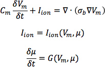
where σbis the bulk conductivity tensor which is calculated from the bidomain conductivity tensors as described by Potse et al30; Vm is the transmembrane potential; Cm is the membrane specific capacitance; and Iion is the density of the transmembrane current, which in turn depends on Vm and a set of state variables μ describing the dynamics of ionic fluxes across the membrane.For Cm , use a value of 1 μ F/cm2. For σi in normal canine heart models, use longitudinal and transverse conductivity values of 0.34 S/m and 0.06 S/m, respectively. Represent llon by the Greenstein-Winslow ionic models of the canine ventricular myocyte. Decrease the electrical conductivities in canine heart failure ventricular models by 30% (Figure 9).
- Using the software package CARP (CardioSolv, LLC), simulate sinus rhythm with all models. Induce reentrant ventricular tachycardia (VT) in the six failing models using an S1-S2 pacing protocol. Choose the timing between S1 and S2 to obtain sustained VT activity for 2 sec after S2 delivery. If VT is not induced for any S1-S2 timing, decrease the conductivities by up to 70% until VT was induced (Figure 10).
- For each simulation, calculate pseudo-ECGs by taking the difference of extracellular potentials between two points in an isotropic bath surrounding the hearts. Place the two points near the base of the heart separated by 18 cm, such that the line connecting them is perpendicular to the base-apex plane of the septum as illustrated in Figure 10. For each simulation with estimated fiber orientations, compute the MAD metric as
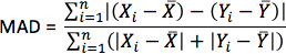
where X is the ECG waveform of the simulation with estimated fiber orientations, Y is the ECG waveform of thecorresponding simulation with acquired fiber orientations, X is the mean value of X,Y is the mean value of Y, and n is the length of X and Y.
Figure 11, A-C displays streamlined visualizations of estimated as well as DTMRI-derived fiber orientations in normal and failing hearts. Qualitative examination shows that estimated fiber orientations align well with DTMRI-derived ones. Panel D illustrates, overlaid on the geometry of heart 1, the distribution of error in normal hearts’ inclination angles, averaged across all five estimates. Panel E shows the mean distribution of error in failing hearts’ inclination angles, overlaid on the geometry of heart 1. Note that inclination angles have values between -90 ° and +90 °, and therefore, the estimation error ranges between 0 ° and 180 °. Panels F and G present sections of tissue from the distributions in panels D and E, respectively. This highlights the transmural variation of error. The histograms of errors in panel H suggest that most myocardial voxels have small error values. About 80% and 75% of the voxels have errors less than 20 ° in normal and failing ventricles, respectively. It was found that the mean error, averaged across all estimated datasets, and all image voxels that belonged to the myocardium, were 14.4 ° and 16.9 ° in normal and failing ventricles, respectively. The mean error in the entire myocardium, in normal and failing cases combined, was 15.4 °. The mean 3D acute angle between estimated and acquired fiber directions were 17.5 ° and 18.8 ° in normal and failing ventricles, respectively. The 3-D angles are comparable to the estimation errors.These results show that inclination angles of predicted fiber orientations are comparable to those acquired by ex-vivo DTMRI, the state-of-the-art technique.The standard deviation of error across the fivedifferent estimates of the fiber orientations of heart 1 was only 1.9 indicating that the variation in estimation quality from oneatlas to another is small.
Figures 12 and 13 present the simulated activation maps of one beat of sinus rhythm activation in normal and failing ventricular models, respectively. Models with estimated fiber orientations produce activation maps very similar to those of models with acquired orientations; the earliest epicardial activations occur at the same sites, and the directions of propagation match as well. The overall mean difference in total activation times between the acquired and estimated fiber orientation cases in the normal ventricular models, averaged over all estimates and all mesh nodes, was 5.7 ms, which is a small fraction (3.7% on average) of the total activation time. Figure 12C demonstrates that pseudo-ECGs obtained for sinus rhythm simulations with models 1 and 3 have identical morphologies. The MAD score between these two waveforms was 4.14%. On average, the MAD score between sinus rhythm pseudo-ECGs with each of models 2 to 6 and model 1 was 10.9%.In simulations of sinus rhythm with failing ventricular models, the mean difference in total activation times between models with acquired and estimated fiber orientations was only 5.2 ms (3.1%), while the mean MAD score was 4.68%. These results indicate that the outcomes of simulation of ventricular activation in sinus rhythm in normal and failing canine ventricular models with fiber orientations estimated with the present methodology closely match those with acquired orientations. In particular, presence of heart failure did not diminish the accuracy of the estimation.
Figure 14 shows simulated activation maps, in apical views of the ventricles, during one cycle of induced VT in the heart failure models, and corresponding pseudo-ECGs. Simulations with acquired and estimated fiber orientation both exhibit similar figure-of-eight reentrant patterns. The ECG morphologies corresponding to estimated and acquired fiber orientations were in good agreement. The mean MAD score was 9.3%. These results indicate that canine heart failure models with estimated fiber orientations can closely replicate outcomes of VT simulations performed using acquired fiber orientations.
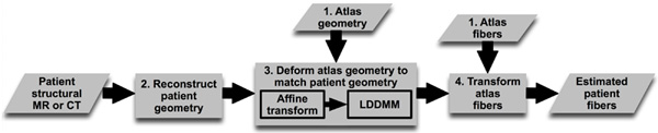
Figure 1. Our processing pipeline for estimating ventricular fiber orientations in vivo. Click here to view larger figure.
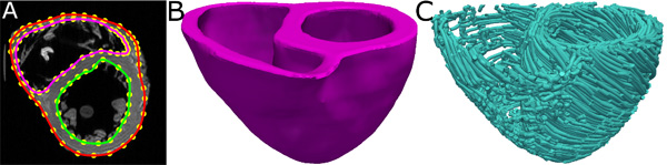
Figure 2. Geometry and fiber orientations of the atlas ventricles. (A) The epicardial (red) and endocardial (green and magenta) splines, and corresponding landmarks (yellow) overlaid on an example slice of the atlas image. (B) The atlas ventricles in 3D. (C) The atlas fiber orientations.
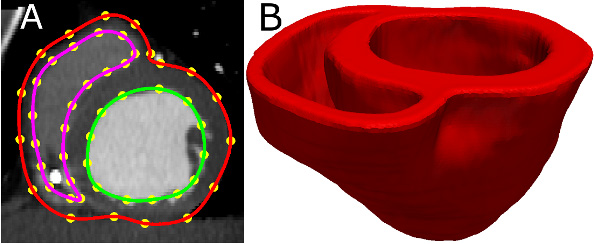
Figure 3. Patient ventricular geometry reconstruction. (A) The epicardial (red) and endocardial (green and magenta) splines, and corresponding landmarks (yellow) overlaid on an image slice. (B) Patient ventricles in 3D.
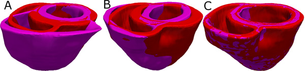
Figure 4. Deformation of the atlas ventricles to match the patient ventricles. (A) Superimposition of ventricles of atlas (magenta, see Figure 2B) and patient (red, see Figure 3B). (B) Patient ventricles and the affine transformed atlas ventricles. (C) Patient ventricles and LDDMM-transformed atlas ventricles.
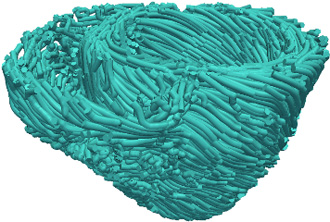
Figure 5. Estimated fiber orientations of the patient heart in Figure 3B.
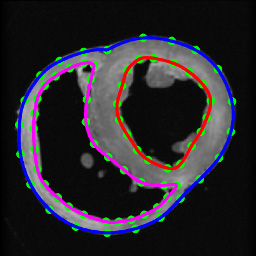
Figure 6. Segmentation of canine hearts. The epicardial (blue) and endocardial (red and magenta) splines, and corresponding landmarks (green) overlaid on an example slice of a normal canine heart.
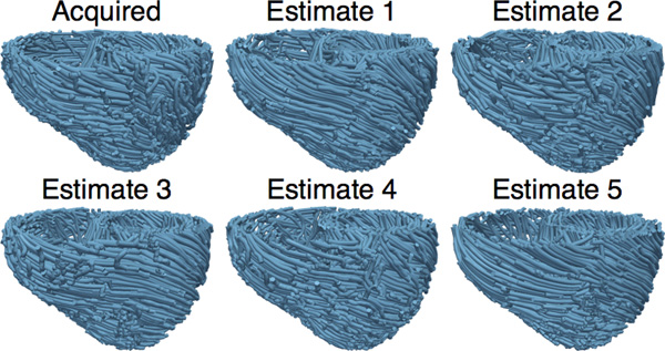
Figure 7. The acquired and estimated fiber orientations of heart 1.
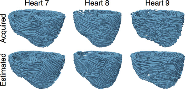
Figure 8. The acquired and estimated fiber orientations of hearts 7-9.
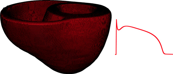
Figure 9. Left panel illustrates the computational mesh generated for the models of heart 1. On the right, the action potential curve of normal canine ventricular myocardium computed using the Greenstein-Winslow model is displayed.
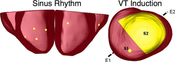
Figure 10. Pacing sites of the simulation of sinus rhythm and VT, as overlaid on the geometry of heart 7. E1E2 illustrates the lead vector used in pseudo-ECG calculations.
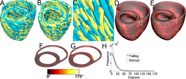
Figure 11. Validation of the fiber orientation estimation methodology by comparing estimated fiber orientations with DTMRI-derived orientations. (A) Superimposition of DTMRI-acquired fiber orientations (greenish yellow) and one set of estimated fiber orientations (cyan) of heart 1. (B) Acquired and estimated fiber orientations of heart 7. (C) An enlarged portion of (B) showing alignment between acquired and estimated fiber orientations. Note that the streamlines were generated at random locations within the myocardium for visualization purposes only, and so their exact positions are irrelevant. (D) Distribution of mean estimation error in normal ventricles. (E) Distribution of mean estimation error in failing ventricles. (F) A section of tissue extracted from (D). (G) A section of tissue extracted from (E). The colorbar applies to D-G. (H) Histograms of errors in normal and failing ventricles. Frequency denotes the number of voxels having a given error.
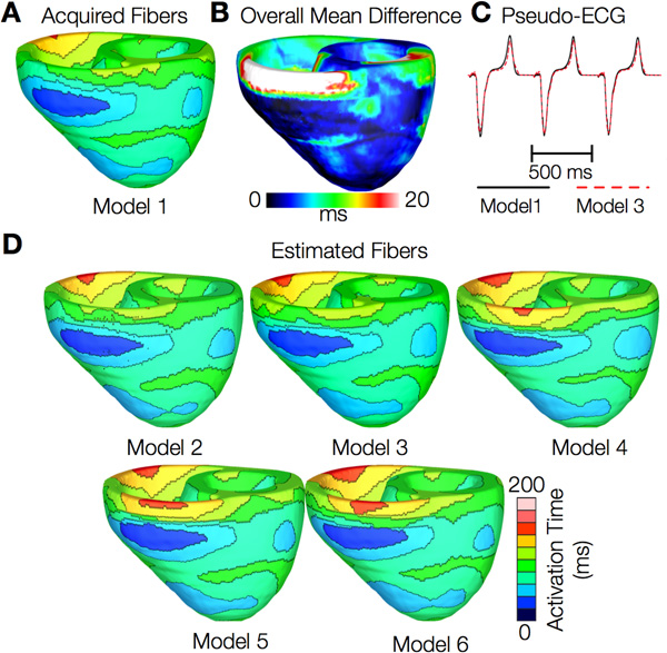
Figure 12. Results from simulations of one beat of sinus rhythm in normal canine ventricular models. (A) Activation map simulated using the model with acquired fiber orientations (model 1). (B) Absolute difference between simulated activation maps obtained from a ventricular model with acquired fiber orientations and that with estimated fiber orientations, averaged over the five estimates. (C) Simulated pseudo-ECGs with models 1 and 3. (D) Simulated activation maps from ventricles with estimated fiber orientations (models 2-6).
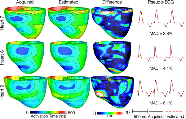
Figure 13. Results from simulations of one beat of sinus rhythm in failing heart models. In th
e first column, rows 1-3 show activation maps calculated using models 7-9, respectively. In the second column, rows 1-3 display results of simulations with models 10-12, respectively. Rows 1-3 in the third column portray the absolute difference between the activation maps shown in the first and second columns of the corresponding row. Rows in the fourth column display simulated pseudo-ECGs from models in the first and second columns of the corresponding row.
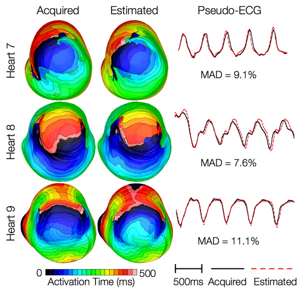
Figure 14. Results from simulations of VT induction with the failing heart models. Rows 1-3 in the first column show activation maps during one cycle of reentrant activity in simulations with models 7-9, respectively. Rows 1-3 in the second column show activation maps corresponding to models 10-12, respectively. Rows in the third column illustrate pseudo-ECGs from models in the first and second columns of the corresponding row.