Note: Brillouin spectral analysis requires a single-longitudinal mode laser (~10 mW at the sample). For aligning purposes, use a strongly attenuated portion of this laser beam (<0.1 mW).
1. Initial Setup of Fiber and the EMCCD (Electron Multiplied Charge Coupled Device) Camera
- Identify about 1,600 mm free aligning space for the spectrometer on an optical table.
- Mount the EMCCD camera at the end of the free aligning space.
- Use set screws to attach the camera to posts. Tighten the posts in post holders at the desired optical axis height. Tighten the post holders onto the optical table using table clamps.
- Turn on the EMCCD camera. Be mindful to avoid camera saturation.
- Install camera software on lab computer and connect the camera to the computer.
- Disable the gain and set low integration time (~0.01 sec). Start acquiring EMCCD images. Observe the camera images on the computer screen.
- Mount the fiber collimator about 1,600 mm in front of the camera.
- Place the fiber collimator in the fiber collimator adapter.
- Mount the adapter onto a post. Tighten the post into a post holder at the approximate height of the optical axis (height of the camera). Tighten post holder onto optical table using table clamps.
- Align the output beam along the optical axis.
- Use a set screw to connect a standard iris to a post. Tighten the post into a post holder.
- Place the iris in front of the fiber collimator (<50 mm). Adjust the height of the iris to the beam. Move the iris along the desired optical axis, which should point directly into the camera.
- Insert an optical density filter directly after the laser output if the camera saturates. Use the adjustment screws of the fiber collimator mount to align the beam along the optical axis. Once this is achieved, the beam will cleanly pass through the iris along the entire beam path.
- Mount a matched achromatic lens pair (f=30 mm) in front of the camera.
2. Horizontal Stage of Spectrometer
- Mount the horizontal mask.
- Use set screws to attach the horizontal mask onto a post. Tighten the post into a post holder. Mount the post holder onto a translational stage, allowing the mask to slide horizontally in and out of the beam path. (Figure 1)
- Use cap screws to tighten the translational stage on the optical table such that the mask is imaged sharply onto the CCD camera at the focal distance (f=30 mm) of the achromatic lens pair.
- Mount and align the spherical lens S1 (f=200 mm) 600 mm in front of the horizontal mask.
- Use set screws to mount S1 onto a post holder. Tighten the post into a post holder.
- Mount two irises as described in 1.5.1. Before placing S1 in the beam path, insert one iris before and one iris after the desired S1 position (600 mm in front of the horizontal mask). Adjust the height of the irises such that the beam cleanly passes through both of them.
- Place S1 600 mm in front of the horizontal mask (Figure 1). Adjust height and angle of S1 until both, the back reflection off of the lens and the out-coming beam, cleanly pass through the irises. Tighten the post holder holding S1 onto the optical table using table clamps.
- Mount VIPA2 in the focal plane of the spherical lens (200 mm in front of S1).
- Mount the VIPA holder onto a post using the screws provided with the holder. Tighten the post into a post holder. Tighten the post holder onto a horizontal translation stage. (Figure 1)
- Place VIPA2 carefully in the VIPA holder with the entrance slit oriented vertically. (Figure 1)
- Fine-adjust the position of the VIPA mount to be exactly in the focal plane of S1. (Check by tracing the beam waist with a white card.)
- Use cap screws to tighten the translational stage onto the optical table and slide VIPA2 out of the beam using the degree of freedom of the translational stage.
- Mount and align the spherical lens S2 (f=200 mm) 200 mm after the VIPA and 200 mm in front of the horizontal mask. Follow the procedure described in 2.2.1-2.2.3. Instead of attaching the post holder onto the optical table, mount it onto a translational stage with its degree of freedom oriented along the optical axis. (Figure 1) Use cap screws to tighten the translational stage onto the optical table.
- Use the horizontal translational stage (2.3.4) to slide the VIPA2 entrance into the beam path. Observe vertical lines on the camera image.
- Fine-adjust S2 using the translational stage mounted in 2.4 until the vertical lines on the camera image appear sharp.
- Adjust the spectrum with the horizontal-tilt degree of freedom on the VIPA holder and the translational stage. Use the horizontal-translation degree of freedom to tune the entrance position of the beam into the etalon. Use the horizontal-tilt degree of freedom to tune the input angle of the beam into the etalon.
- Measure finesse and throughput.
- Take an image by pressing F5 or alternatively by clicking “acquisition setup” in the upper left hand corner and choosing the option “take image” in the camera software.
- Right click on the image and choose the option “line plot”. Drag the cursor horizontally across the image to generate a line plot. Release the cursor to observe the generated line plot.
- Use the line plot to measure the finesse. Divide the distance between two peaks by their full width at half maximum (FWHM). Aim for >30.
- Determine the throughput by measuring the power with a power meter immediately before and after VIPA2. Aim for >50%.
- Tune the input angle of the beam into the etalon with the degree of freedom on the VIPA holder (2.6) and observe the trade-off between finesse and throughput.
- If finesse and throughput are not satisfactory go back and fine-adjust the alignment. Make sure VIPA2 is in the focal plane of S1. Repeat steps 2.3.3 -2.7.
3. Vertical Stage of Spectrometer
- Slide the VIPA (VIPA2), aligned in part 2, out of the beam using the translational stage (2.3.4). The horizontal stage of the spectrometer will now behave as a 1:1 imaging system.
- Mount the vertical mask.
- Use set screws to attach the vertical mask onto a post. Tighten a post into a right angle post clamp adapter. Tighten a second post into the right angle adapter and put it into a post holder. Mount the post holder onto a vertical translational stage, allowing the mask to slide vertically in and out of the beam path. (Figure 1)
- Use cap screws to tighten the vertical translational stage onto the optical table such that the vertical mask is imaged sharply onto the EMCCD camera 200 mm in front of S1.
- Mount and align the cylindrical lens C1 (f=200 mm) 600 mm in front of the vertical mask.
- Screw the cylindrical lens holder onto a post. Tighten the post into a post holder. Carefully place C1 into the lens holder and tighten the screws to fix it in place.
- Mount two irises as described in 1.5.1. Before placing C1 in the beam path, insert one iris before and one iris after the desired S1 position (600 mm in front of the vertical mask). Adjust the height of the irises such that the beam cleanly passes through both of them.
- Place C1 600 mm in front of the vertical mask (Figure 1). Carefully adjust the height, tilt, and lateral position of C1 until both, the back reflection off of the lens and the out-coming beam, are centered onto the irises. Tighten the post holder holding C1 onto the optical table using table clamps.
- Mount VIPA1 in the focal plane of the cylindrical lens (200 mm in front of C1).
- Mount the VIPA holder onto a post using the screw provided with the holder. Tighten the post into a post holder. Tighten the post holder onto a vertical translation stage. (Figure 1)
- Place VIPA1 carefully into the VIPA holder with the entrance slit oriented horizontally. (Figure 1)
- Fine-adjust the position of the VIPA mount to place VIPA1 exactly in the focal plane of C1. (Check by tracing the beam waist with a white card.)
- Use cap screws to tighten the vertical translational stage onto the optical table and slide VIPA1 out of the beam using the degree of freedom of the translational stage.
- Mount and align the cylindrical lens C2 (f=200 mm) 200 mm after VIPA1 and 200 mm in front of the vertical mask, following the procedure described in 3.3.1-3.3.3. Instead of attaching the post holder onto the optical table, mount it onto a translational stage with its degree of freedom oriented along the optical axis. (Figure 1) Use cap screws to tighten the translational stage onto the optical table.
- Use the translation stage (3.4.4) to slide the VIPA1 entrance into the beam path. Observe horizontal lines on the camera image.
- Fine-adjust C2 using the translational stage mounted in 3.5 until the horizontal lines on the camera image appear sharp.
- Adjust the spectrum with the vertical-tilt degree of freedom on the VIPA holder and the translational stage. Use the vertical-translation degree of freedom to tune the entrance position of the beam into the etalon. Use the vertical-tilt degree of freedom to tune the input angle of the beam into the etalon.
- Measure finesse and throughput.
- Follow steps 2.7.1 -2.7.2 to generate a line plot vertically across an image of the camera screen.
- Use the line plot to measure the finesse by dividing the distance between two horizontal lines by their full width at half maximum (FWHM). Aim for > 40.
- Measure the throughput by measuring the power with a power meter immediately before and after VIPA1. Aim for >30%.
- Tune the vertical input angle of the beam into the etalon with the vertical-tilt degree of freedom on the VIPA holder (3.7). Observe the trade-off between finesse and throughput.
- If finesse and throughput are not satisfactory go back and fine-adjust the alignment. Make sure VIPA1 is in the focal plane of C1. Repeat step 3.4.3-3.8.
4. Combination of the Two Stages and Final Alignment
- Slide in VIPA2. Observe horizontally and vertically spaced dots. These dots are the spectral signature of the single frequency laser. Adjust the translational stages of the VIPAs until the dots are in sharp focus.
- Measure finesse and throughput of the spectrometer.
- Follow steps 2.7.1.-2.7.2 to generate a line plot diagonally across two of the laser dots.
- Use the line plot to measure finesse by dividing the diagonal distance between two dots by their full width at half maximum (FWHM). Aim for >30.
- Build a black box to enclose the spectrometer.
- Use construction rails to build the box skeleton, which should enclose the entire spectrometer from the fiber collimator to the CCD camera (63 in x 9 in x 15 in).
- Cover the box skeleton with Blackout Fabric and tape it tight at the corners. Ensure that the masks and the VIPAs are easily accessible.
- Connect the fiber to a standard optical probe, such as a reflectance confocal microscope4. Standard optical probes used to collect back-scattered light will carry a Brillouin signal.
5. Measuring the Brillouin Shift
- Close both the vertical and the horizontal masks until the laser signature disappears. Move the translation stages accordingly.
- Enable the gain and increase the integration time of the camera as much as possible without saturating the EMCCD camera.
- Observe the Brillouin shift of a sample.
- Place a sample in the focus of a confocal microscope (or other optical probe). The spatial resolution will depend on the objective lens used in the confocal microscope. Use a plastic dish or a cuvette for liquids. Use Methanol for the first measurement.
- To optimize the spectrometer throughput, open one mask at a time and scan through the spectrometer orders by tilting the VIPA and adjusting its translation stage. Find the order in which the signal appears the strongest. Close mask again until the laser signal disappears. Repeat with the other mask and VIPA (described in 2.6 and 3.7).
- Take a measurement of the sample.
- Take an image of the spectrum following step 2.7.1.
- Obtain calibration measurements by taking an image of the spectrum of water and glass (or other sample with known Brillouin shift). Save the image by clicking “file” in the upper left hand corner and choosing the option “save as”. Save the image in “.sif” format if the data analysis is performed in the camera software. Save the image in “.tif” format if the data analysis is performed in another computational software program.
6. Calibration and Analysis of Brillouin Spectrum
- Determine the free spectral range (FSR) and the EMCCD pixel to optical frequency conversion ratio (PR) in the Brillouin spectrometer.
- Load the data in the camera software or another computational software program.
- Follow step 2.7.2 to generate a line plot across the spectrum of the water calibration image.
- Fit the two peaks of the spectrum with Lorentzian curves to determine peak positions in terms of pixel position (PWater-S, PWater-AS). Alternatively, read out the peak positions manually by taking the highest point of the peaks.
- Repeat step 6.1.2-6.1.3 with the spectrum of the glass calibration image.
- Alternatively to 6.1.1-6.1.4, add both EMCCD frames and fit all four peaks at once. (Figure 2)
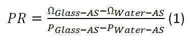
- Calculate the PR using equation 1. Plug in the values for PWater-AS and PGlass-AS determined in 6.1.3 and 6.1.4. ΩGlass-AS is known to be 29.3 GHz. In this case, since the free spectral range is only 20 GHz it will appear aliased with the frequency shift of 9.3 GHz. For simplicity use 9.3 GHz for ΩGlass-AS. Use 7.46 GHz for ΩWater-AS.
- Calculate the FSR using equation 2. Plug in the values for PGlass-S, PGlass-AS and PR, calculated in 6.16. Use 9.3 GHz for ΩGlass-AS.
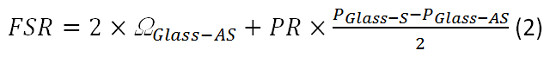
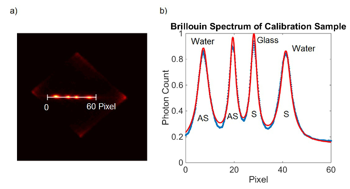
Figure 2. Spectrometer calibration. (A) EMCCD camera frame obtained from calibration sample. (B) Lorentzian curve fit (red) to the measured data (blue). Please click here to view a larger version of this figure.
- Determine the Brillouin shift of a sample.
- Follow step 2.7.2 to generate a line scan across the spectrum of the sample.
- Fit the two peaks of the spectrum with Lorentzian curves to determine peak positions in terms of pixel position. Alternatively, read out the peak positions manually by taking the highest point of the peaks.
- Use the following equations 4 and 5 and the previously calculated values for FSR and PR to calculate the Brillouin shift of the sample.
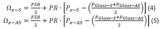
Figure 3 shows representative Brillouin spectra and their fits for different materials. The VIPAs both have a thickness of 5 mm which results in a FSR of approximately 20 GHz. The integration time for these measurements was 100 msec. 100 measurements were taken and averaged. One calibration measurement was taken prior to acquiring the spectra.
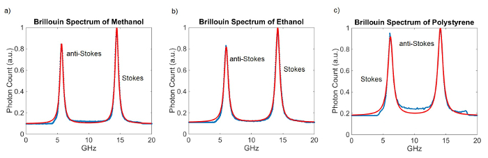
Figure 3. Brillouin Spectra of different materials. Lorentzian curve fit (red) to the measured data (blue). (a) Brillouin spectrum of Methanol. The measured Brillouin shift is 5.59 GHz. (b) Brillouin spectrum of Ethanol. The measured Brillouin shift is 5.85 GHz. (c) Brillouin spectrum of Polystyrene. The measured Brillouin shift is 14.12 GHz. Please click here to view a larger version of this figure.
The obtained Brillouin shifts agree with previously published data3,6,7. To determine if the alignment of the spectrometer is optimal, many spectral measurements of the same material can be taken sequentially, and the standard deviation of the peak positions can be calculated. Figure 4A shows a time-trace of 250 Brillouin measurements of methanol taken sequentially; a histogram of the evaluated Brillouin shifts is shown in Figure 4B. A well-aligned spectrometer with 5 mW of light at the sample and an integration time of 100 msec will have a standard deviation of σ ~ 10 MHz. Changes in Brillouin shift within corneal and lens tissue have been measured to be on the order of 1 GHz9,10,11. Therefore, Brillouin shift readings with variability of ≤10 MHz will enable the measurement of relevant mechanical variations in tissue.
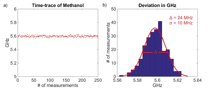
Figure 4. Deviation in Brillouin shift over 250 methanol measurements. (A) Time-trace of 250 Brillouin measurements of methanol. (B) Histogram of Brillouin shift deviation over 250 measurements. Please click here to view a larger version of this figure.