Using the Open-Source MALDI TOF-MS IDBac Pipeline for Analysis of Microbial Protein and Specialized Metabolite Data

Summary

IDBac is an open-source mass spectrometry-based bioinformatics pipeline that integrates data from both intact protein and specialized metabolite spectra, collected on cell material scraped from bacterial colonies. The pipeline allows researchers to rapidly organize hundreds to thousands of bacterial colonies into putative taxonomic groups, and further differentiate them based on specialized metabolite production.

Abstract

In order to visualize the relationship between bacterial phylogeny and specialized metabolite production of bacterial colonies growing on nutrient agar, we developed IDBac—a low-cost and high-throughput matrix-assisted laser desorption/ionization time-of-flight mass spectrometry (MALDI-TOF MS) bioinformatics pipeline. IDBac software is designed for non-experts, is freely available, and capable of analyzing a few to thousands of bacterial colonies. Here, we present procedures for the preparation of bacterial colonies for MALDI-TOF MS analysis, MS instrument operation, and data processing and visualization in IDBac. In particular, we instruct users how to cluster bacteria into dendrograms based on protein MS fingerprints and interactively create Metabolite Association Networks (MANs) from specialized metabolite data.

Introduction

A major barrier to researchers who study bacterial function is the ability to quickly and simultaneously assess the taxonomic identity of a microorganism and its capacity to produce specialized metabolites. This has prevented significant advances in understanding the relationship between bacterial phylogeny and specialized metabolite production in the majority of bacteria isolated from the environment. Although MS-based methods that use protein fingerprints to group and identify bacteria are well described^1,2,3,4, these studies have generally been performed on small groups of isolates, in a species-specific manner. Importantly, information on specialized metabolite production, a major driver of microbial function in the environment, has remained unincorporated in these studies. Silva et al.⁵ recently provided a comprehensive history detailing the underuse of MALDI-TOF MS to analyze specialized metabolites and the shortage of software to relieve current bioinformatics bottlenecks. In order to address these shortcomings, we created IDBac, a bioinformatics pipeline that integrates both linear and reflectron modes of MALDI-TOF MS⁶. This allows users to rapidly visualize and differentiate bacterial isolates based on both protein and specialized metabolite MS fingerprints, respectively.

IDBac is cost-effective, high-throughput, and designed for the lay user. It is freely available (chasemc.github.io/IDBac), and only requires access to a MALDI-TOF mass spectrometer (reflectron mode will be required for specialized metabolite analysis). Sample preparation relies on the simple “extended direct transfer” method^7,8 and data are collected with consecutive linear and reflectron acquisitions on a single MALDI-target spot. With IDBac, it is possible to analyze the putative phylogeny and specialized metabolite production of hundreds of colonies in under four hours, including sample preparation, data acquisition, and data visualization. This presents a significant time and cost advantage over traditional methods of identifying bacteria (such as gene sequencing), and analyzing metabolic output (liquid chromatography-mass spectrometry [LCMS] and similar chromatographic methods).

Using data obtained in linear mode analysis, IDBac employs hierarchical clustering to represent the relatedness of protein spectra. Since the spectra mostly represent ionized ribosomal proteins, they provide a representation of the phylogenetic diversity present in a sample. In addition, IDBac incorporates reflectron mode data to display specialized metabolite fingerprints as Metabolite Association Networks (MANs). MANs are bipartite networks that allow for easy visualization of shared and unique metabolite production between bacterial isolates. The IDBac platform allows researchers to analyze both protein and specialized metabolite data in tandem but also individually if only one data-type is acquired. Importantly, IDBac processes raw data from Bruker and Xiamen instruments, as well as txt, tab, csv, mzXML, and mzML. This eliminates the need for manual conversion and formatting of data sets, and significantly reduces the risk of user error or mishandling of MS data. 

Protocol

1. Preparation of MALDI matrix

1. Prepare 10 mg/mL MALDI-grade, and/or recrystallized α-cyano-4-hydroxycinnamic acid (CHCA) in MS-grade solvents: 50% acetonitrile (ACN), 47.5% water (H₂O), 2.5% trifluoroacetic acid (TFA). Example: 100 µL solution = 50 µL ACN + 47.5 µL H₂O + 2.5 µL TFA + 1 mg CHCA
   1. Prepare at least 1 µL of matrix solution per MALDI plate spot and vortex or sonicate until in solution (approximately 5 min sonication or no visible solids).
      CAUTION: TFA is a strong acid that should be handled in a chemical fume hood while wearing proper personal protective equipment, as it can damage skin, eyes, and airways with contact or inhalation.
      NOTE: CHCA is hygroscopic and light-sensitive and should be stored in amber vials in a desiccator. There are many MALDI matrix options available. CHCA is most common for protein profiling of bacteria, but also works for specialized metabolite analysis. Matrix selection depends on individual user/experiment needs.

2. Preparation of MALDI target plates

NOTE: See Sauer et al.⁷, for more details.

1. Rinse MALDI plate with methanol (HPLC-grade or higher) and wipe dry with soft paper wipes. Do not use abrasive brushes when cleaning target plates, as this can permanently damage the surface of the target plate.
2. Assign protein and specialized metabolite calibrant spots. Organize calibration spots evenly across the sample population, to account for MALDI-plate-irregularities and instrument drift over time. Assign an appropriate number of media/matrix-blank spots for the study; these spots will contain only media and matrix, or only matrix.
3. Using a sterile toothpick, transfer a small portion of a bacterial colony to the appropriate spot on the MALDI plate. Spread the bacterial colony evenly over the spot. The spot should appear as flat as possible.
   NOTE: It will be easier to flatten bacterial colonies that are more mucoid/amorphous. For more rigid/solid colonies, avoid leaving visible clusters of cell mass on the MALDI spot (Figure 1).

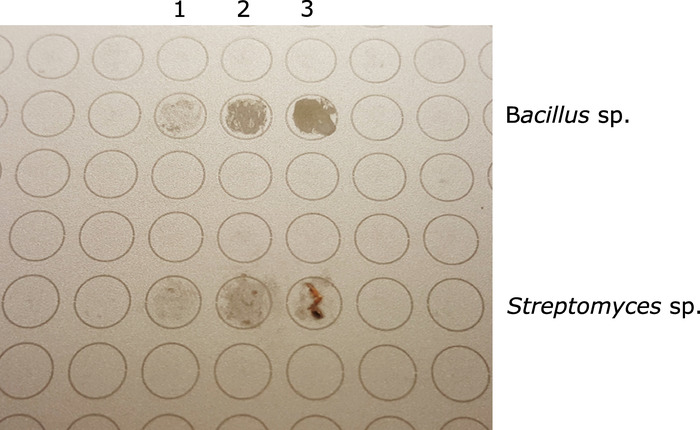
Figure 1: MALDI-target plate showing two different isolates before adding formic acid and MALDI matrix (top 3 spots - Bacillus sp.; bottom 3 spots - Streptomyces sp.). For both, column 3 represents excess sample; column 2 represents the appropriate amount of sample; column 1 represents insufficient sample for MALDI analysis. Please click here to view a larger version of this figure.

4. Prepare a matrix/media control by using a sterile toothpick to transfer a minimal amount of agar/media onto the appropriate spot(s) on the MALDI plate.
5. Overlay 1 µL of 70% mass spectrometry grade formic acid onto each sample spot, including the matrix control spots. Allow acid to air dry completely in a chemical fume hood (approximately 5 min).
   CAUTION: Formic acid is a caustic chemical and should be handled in chemical fume hoods. It can damage airways if inhaled.
6. Add 1 µL of the prepared MALDI matrix solution to each sample spot, as well as to the matrix/media control spots. Allow matrix solution to air dry completely (approximately 5 min).
   NOTE: It is possible to store the plate in a desiccator, in the dark, until it can be analyzed on a MALDI-TOF mass spectrometer. Allowable storage times may vary depending on sample stability.
7. Add 0.5–1.0 µL calibrant to the assigned calibration spots, followed by 1 µL MALDI matrix solution. Pipette the resulting solution up and down to mix. Allow all spots to air dry completely prior to introduction into the MALDI-TOF mass spectrometer.
   NOTE: The protein and specialized metabolite calibrants should be added within 30 min of MALDI analysis, as both are susceptible to degradation.

3. Data acquisition

NOTE: The general parameters for data acquisition are listed in Table 1.

Parameter	Protein	Specialized Metabolite
Mass Start (Da)	1920	60
Mass End (Da)	21000	2700
Mass Deflection (Da)	1900	50
Shots	500	1000
Frequency (Hz)	2000	2000
Laser Size	Large	Medium
MaxStdDev (ppm)	300	30

Table 1.

1. Following the protocols specific to the instrument being used, set up both protein and specialized metabolite calibrations.
2. Test a few separate target spots to determine the optimal laser power and detector gain to use when acquiring spectra (this will vary day-to-day and by instrument).
   NOTE: Figure 2A and Figure 3A show optimal spectra, while Figure 2D and Figure 3D are examples of poor-quality spectra.

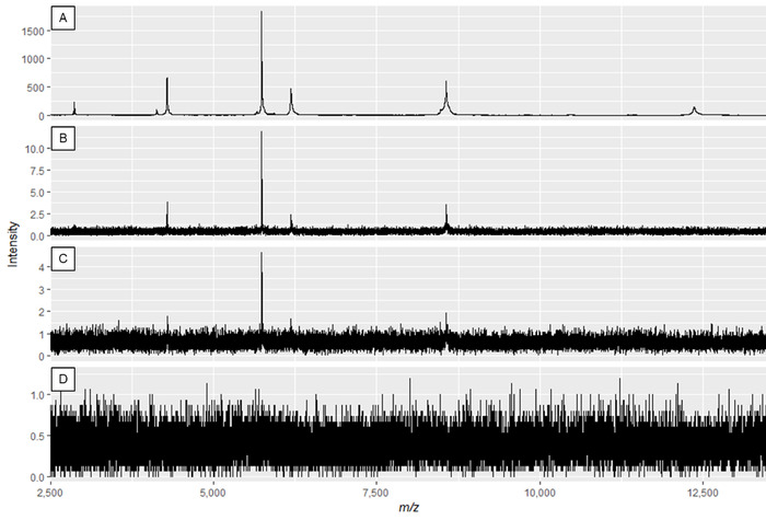
Figure 2: Example protein spectra displaying the effect of modifying laser power and detector gain. Spectra quality is best in panel A, and decreases until insufficient spectra quality in panels C and D. While the spectrum in panel B may result in useable peaks, panel A displays optimal data. Please click here to view a larger version of this figure.

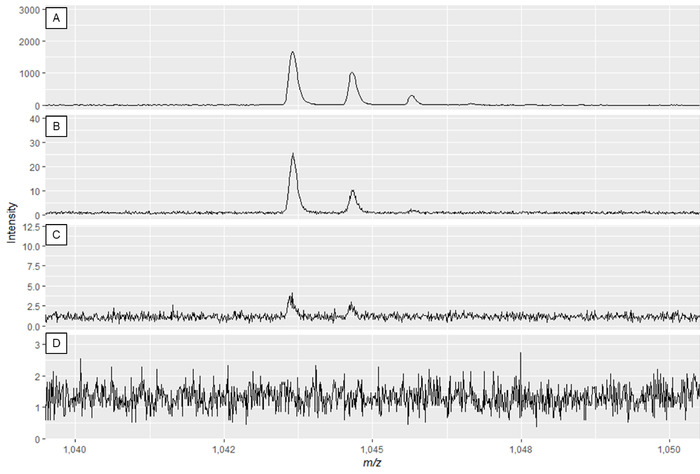
Figure 3: Example specialized metabolite spectra displaying the effect of modifying laser power and detector gain. Spectra quality is best in panel A and decreases until insufficient spectra quality in panels C and D. While the spectrum in panel B may result in useable peaks, panel A displays optimal data. Please click here to view a larger version of this figure.

3. Acquire spectra, saving protein spectra into one folder and specialized metabolite spectra into a second, separate folder.

4. Cleaning the MALDI target plate (adapted from Sauer et al.⁷)

1. Remove the MALDI target plate from its holder and rinse with acetone.
2. Wash with a non-abrasive liquid soap to remove trace proteins and lipids, and soft paper wipes/soft-bristled toothbrush.
3. Rinse with de-ionized water for approximately 2 min to completely remove soap.
4. Sonicate the target plate in water (HPLC grade or higher) for 5 min.
5. Rinse the target plate with water (HPLC grade or higher).
6. Rinse the target plate with methanol (HPLC grade or higher).

5. Installing the IDBac Software

1. Download the IDBac software.
   NOTE: Permanent, versioned backups are also available for download (see the Table of Materials).
2. Double-click the downloaded “Install_IDBac.exe” to initiate the installer and follow the on-screen instructions.

6. Starting with Raw Data

NOTE: Detailed explanations and instructions of each data processing step are embedded within IDBac, however the main analyses and interactive inputs are described below.

1. Double-click the IDBac desktop shortcut to launch IDBac. IDBac will open on the Introduction tab by default.
2. Use the Check for Updates button to ensure that the most current version of IDBac is being used (requires internet access). If a newer version is available, IDBac will automatically download and install the update, after which IDBac will request to be restarted.
3. Click on the Starting with Raw Data tab and choose from the menu the type of data to be used with IDBac; continue by following the in-app instructions.
4. When setting-up the conversion and processing of data files, input a descriptive name for the experiment where prompted (see Figure 4). Experiments will later be displayed alphabetically, so a helpful strategy is to start experiment names with a group-attribute (e.g., “bacillus-trials_experiment-1”; “bacillus-trials_experiment-2”).

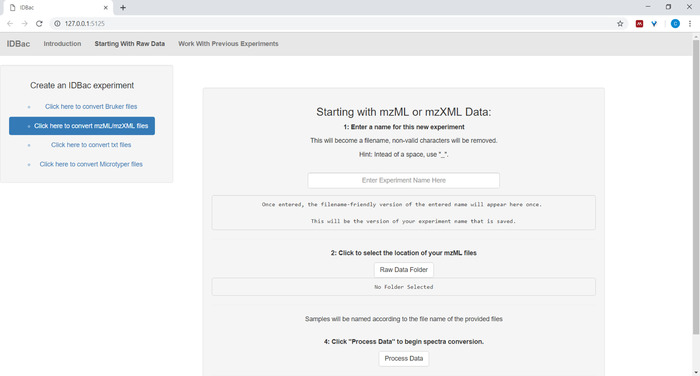
Figure 4: IDBac data conversion and preprocessing step. IDBac converts raw spectra into the open mzML format and stores mzML, peak lists, and sample information in a database for each experiment. Please click here to view a larger version of this figure.

7. Work with previous experiments

1. After converting files and processing them with IDBac, or anytime one wishes to reanalyze an experiment, navigate to the Work with previous experiments page and Select an experiment to work with (Figure 5).

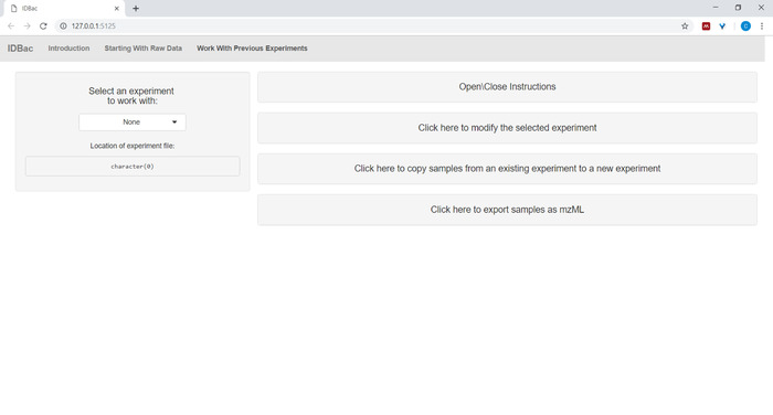
Figure 5: "Work with Previous Experiments" page. Use IDBac’s “Work with Previous Experiments” page to select an experiment to analyze or modify. Please click here to view a larger version of this figure.

2. (Optional) Add information about samples using the menu Click here to modify the selected experiment. Input information into the auto-populated spreadsheet and press Save (Figure 6). This option allows the user to color-code data during analyses.

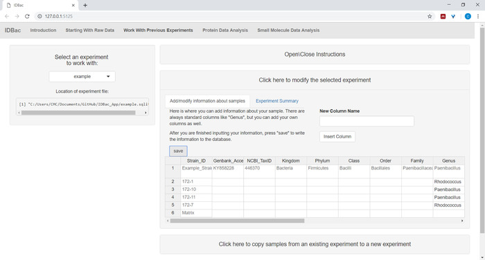
Figure 6: Input sample information. Within the “Work with Previous Experiments” page users can input information about samples such as taxonomic identity, collection location, isolation conditions, etc. Please click here to view a larger version of this figure.

3. (Optional) Transfer all, or a subset of samples to a new or another experiment by clicking Transfer samples from previous experiments to new/other experiments and following the provided instructions (Figure 7).

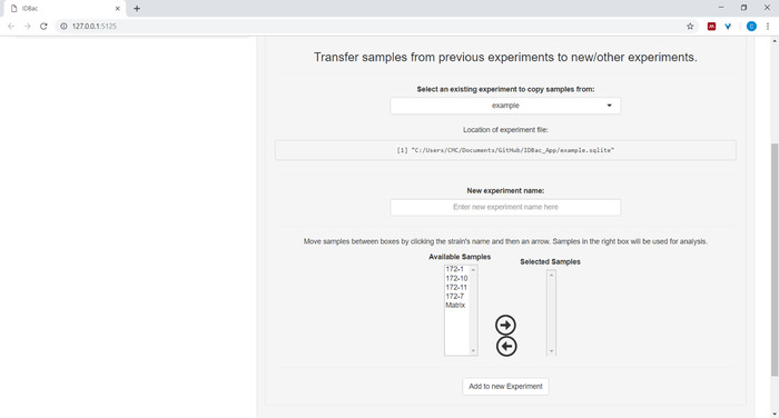
Figure 7: Transfer data. The “Work with Previous Experiments” page contains the option to transfer data between existing experiments and to new experiments. Please click here to view a larger version of this figure.

4. When ready to begin analysis, ensure the experiment to work with is selected. Select either Protein Data Analysis or Small Molecule Data Analysis.

8. Setting up protein data analysis and creating mirror plots

1. If analyzing protein data, first navigate to the Protein Data Analysis page. Choose peak-picking settings and evaluate protein spectra of samples via the displayed mirror plots (Figure 8).
   NOTE: In the mirror plots, a red peak signifies the presence of that peak only in the top spectrum, while blue peaks represent those occurring in both spectra.

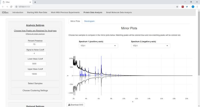
Figure 8: Choose how peaks are retained for analysis. After selecting an experiment to analyze, visiting the “Protein Data Analysis” page and subsequently opening the “Choose how Peaks are Retained for Analysis” menu allows users to choose settings like signal-to-noise ratio for retaining peaks. The displayed mirror plot (or dendrogram) will automatically update to reflect the chosen settings. Please click here to view a larger version of this figure.

2. Adjust the percentage of replicates in which a peak must be present in order for it to be included for analyses (e.g., if the threshold is set to 70% and a peak occurs in at least 7 out of 10 replicates, it will be included).
3. Using the mirror plots as visual guidance, adjust the signal to noise cutoff that retains the most “genuine” peaks and the least noise, noting that more replicates and a higher “percentage peak presence” value will allow selection of a lower signal to noise cutoff.
4. Specify the lower and upper m/z cutoffs, dictating the range of mass values within each spectrum to be used in further analyses by IDBac.

9. Clustering samples using protein data

1. Within the Protein Data Analysis page, select the Dendrogram tab. This allows for grouping samples into a dendrogram according to user-selected distance measures and clustering algorithms.
2. Click Select Samples on the menu and follow the instructions to select samples to include in the analyses. Only samples that contain protein spectra will be displayed within the Available Samples box (Figure 9).

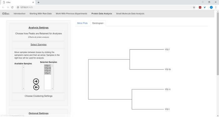
Figure 9: Select samples from the chosen experiment to include within the displayed dendrogram. Please click here to view a larger version of this figure.

3. Use the default values or, under Choose Clustering Settings, select the desired Distance and Clustering algorithms to be applied to the generation of the dendrogram.
4. Select Presence/Absence as input. Alternatively, if confident about the peak heights of the samples (e.g., after performing a study to assess variability of peak intensity), select Intensities as input.
   NOTE: At the time of publication, IDBac provides flexibility in settings for clustering, relying on users to choose the appropriate combinations. If unfamiliar with these options, it is suggested to pair either A: “cosine” distance, and “average (UPGMA)” clustering; or B: “Euclidean” distance, and “Ward.D2” clustering.
5. To display bootstrap values on the dendrogram, enter a number between 2 and 1000 under Bootstraps.
6. When reporting results, copy the text within the Suggestions for Reporting Protein Analysis paragraph. This provides the user-defined settings that generated the specific dendrogram.

10. Customizing the protein dendrogram

1. To begin customizing the dendrogram, open the Adjust the dendrogram menu (Figure 10).

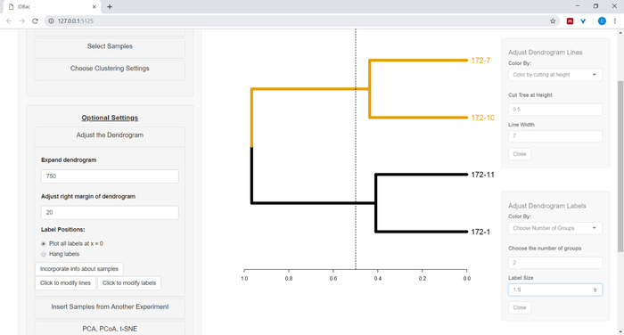
Figure 10: Adjust the dendrogram. IDBac provides a few options for modifying how the dendrogram looks, these may be found within the menu “Adjust the Dendrogram”. This includes coloring branches and labels by k-means, or by “cutting” the dendrogram at a user-provided height. Please click here to view a larger version of this figure.

2. To color the dendrogram’s lines and/or labels select the appropriate button: Click to modify lines or Click to modify labels and select the desired options.
3. To plot information from the spreadsheet next to the dendrogram (see step 7.2), select the button Incorporate info about samples. This will open a panel where a category (column in the spreadsheet) will self-populate based on the entered values (Figure 11).

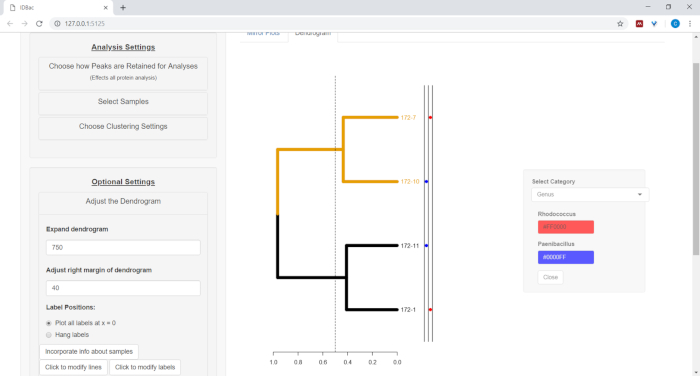
Figure 11: Incorporate info about samples. Within the “Adjust the Dendrogram” menu is the option “Incorporate info about samples”. Selecting this will allow plotting information about samples next to the dendrogram. Sample information is input within the “Work with Previous Experiments” page. Please click here to view a larger version of this figure.

11. Insert samples from a separate experiment into the dendrogram

1. To insert samples from another experiment, select the menu button Insert Samples from Another Experiment. Follow the directions in the newly-opened panel (Figure 12).

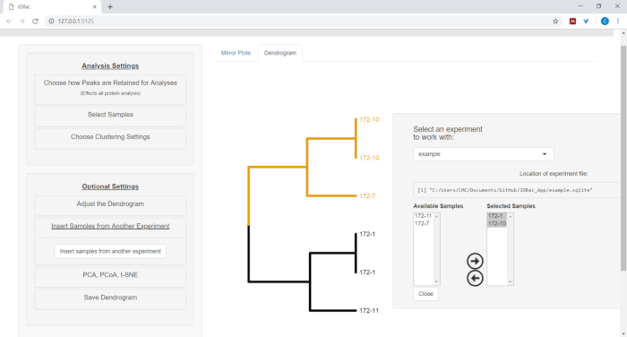
Figure 12: Insert Samples from Another Experiment menu. Sometimes it is helpful to compare samples from another experiment. Use the “Insert Samples from Another Experiment” menu to choose samples to include within the currently-displayed dendrogram. Please click here to view a larger version of this figure.

12. Analyzing specialized metabolite data and metabolite association networks (MANs)

1. Proceed to the Metabolite Association Network (Small-Molecule) page. This page allows for data visualization by principle components analysis (PCA) and MANs, which use bipartite networks to display the correlation of small molecule m/z values with samples.
2. If a protein dendrogram was created (section 9), it will be displayed on this page as well. Click-and-drag on the dendrogram to highlight select samples of interest to be analyzed. If no samples are highlighted or no protein dendrogram was created, a MAN of a either a random subset or all samples will appear, respectfully (Figure 13).

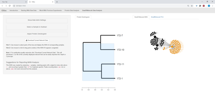
Figure 13: Small Molecule Data Analysis” page. If a dendrogram was created from protein spectra, it will be displayed within the “Small Molecule Data Analysis” page. This page will also display Metabolite Associate Networks (MANs) and Principle Components Analysis (PCA) for small molecule data. Please click here to view a larger version of this figure.

3. To subtract a matrix/media blank in the MAN, open the menu Select a Sample to Subtract and choose the appropriate sample to use as a blank.
4. Open the menu Show/Hide MAN Settings to select the desired values for percentage of peak presence in replicates, signal to noise, and upper and lower mass cutoffs, as was done for protein spectra in Section 9. Use the small molecule mirror plots to guide the selection of these settings.
5. Select “Download Current Network Data” to save the data of the MAN that is currently displayed. These data can be used in network analysis software other than IDBac.
6. For reporting results, copy the text within the Suggestions for Reporting MAN Analysis paragraph. This provides the user-defined settings used to generate the created MAN.

13. Sharing data

1. Each IDBac “experiment” is saved as a single SQLite database. It contains the converted mzML raw spectra, detected peaks, and all user-input information about samples. Therefore, to share an IDBac experiment simply share the SQlite file that has the same name as the experiment (the file location is displayed on the Working with Previous Experiments page).

Results

We analyzed six strains of Micromonospora chokoriensis and two strains of Bacillus subtilis, which were previously characterized⁶, using data available at DOI: 10.5281/zenodo.2574096. Following directions in the Starting with Raw Data tab, we selected the option Click here to convert Bruker files and followed the IDBac-provided instructions for each dataset (Figure 14).

After the automated conversion and preprocessing/peak-peaking steps were completed, we proceeded to create a new combined IDBac experiment by transferring samples from the two experiments into a single experiment containing both Bacillus and Micromonosopora samples (Figure 15). The resulting analysis involved comparing protein spectra using mirror plots, as pictured in Figure 16, which was useful for evaluating spectra quality and adjusting peak-picking settings. Figure 17 displays a screenshot of the protein clustering results with default settings selected. The dendrogram was colored by adjusting the threshold on the plot (appears as a dotted line). Of note is the clear separation between genera, with both M. chokoriensis and B. subtilis isolates clustering separately.

Figure 18, Figure 19, and Figure 20 highlight the ability to generate MANs of user-selected regions by clicking and dragging across the protein dendrogram. With this we were able to rapidly create MANs to compare only the B. subtilis strains (Figure 18), only the M. chokoriensis strains (Figure 19), and all the strains simultaneously (Figure 20). The primary function of these networks is to provide researchers with a broad overview of the degree of specialized metabolite overlap between bacteria. With these data in hand, researchers now have the capacity to make informed decisions from only a small amount of material scraped from a bacterial colony.

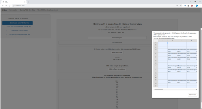
Figure 14: Spectra processing. Downloaded Bruker autoFlex spectra were converted and processed using IDBac. Please click here to view a larger version of this figure.

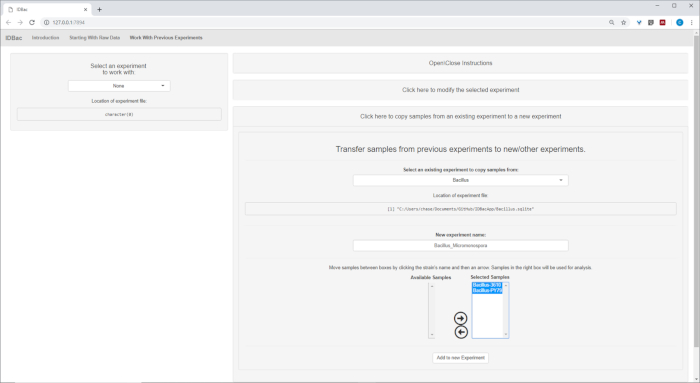
Figure 15: Combined IDBac experiment. Because the Micromonospora and Bacillus spectra were collected on different MALDI target plates, the two experiments were subsequently combined into a single experiment-“Bacillus_Micromonsopora”. This was done within the “Work with Previous Experiments” tab, following directions within the menu “Transfer samples from previous experiments to new/other experiments”. Please click here to view a larger version of this figure.

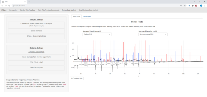
Figure 16: Comparison. Micromonspora and Bacillus spectra were compared using the mirror plots within the “Protein Data Analysis” page. Ultimately, default peak settings were chosen. Please click here to view a larger version of this figure.

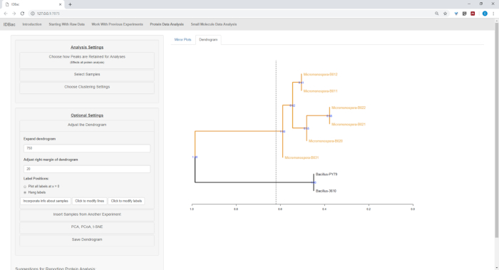
Figure 17: Hierarchical clustering. Hierarchical clustering, using default settings, correctly grouped Bacillus and Micromonospora isolates. The dendrogram was colored by “cutting” the dendrogram at an arbitrary height (displayed as a dashed-line) and 100 bootstraps used to show confidence in branching. Please click here to view a larger version of this figure.

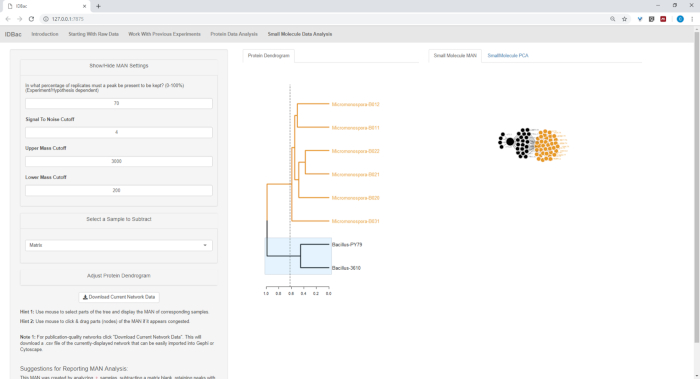
Figure 18: MAN created by selecting the Bacillus sp. strains from the protein dendrogram showed differential production of specialized metabolites. Please click here to view a larger version of this figure.

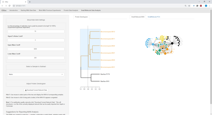
Figure 19: MAN created by selecting the six Micromonospora sp. strains from the protein dendrogram showed differential production of specialized metabolites. Please click here to view a larger version of this figure.

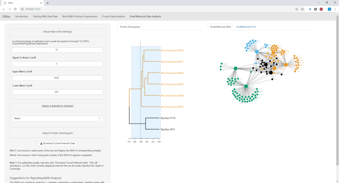
Figure 20: MAN of Bacillus sp. and Micromonospora sp. strains showing a differential production of specialized metabolites. Please click here to view a larger version of this figure.

Discussion

The IDBac protocol details bacterial protein and specialized metabolite data acquisition and analysis of up to 384 bacterial isolates in 4 h by a single researcher. With IDBac there is no need to extract DNA from bacterial isolates or generate specialized metabolite extracts from liquid fermentation broths and analyze them using chromatographic methods. Instead, protein and specialized metabolite data are gathered by simply spreading material from bacterial colonies directly onto a MALDI target plate. This greatly reduces the time and cost associated with alternative techniques such as 16S rRNA gene sequencing and LCMS⁹.

It is important to add a matrix blank and calibration spots to the MALDI plate, and we recommend using an appropriate number of replicates to ensure reproducibility and statistical confidence. The numbers of replicates will be experiment-dependent. For example, if a user intends to differentiate thousands of colonies from a collection of environmental diversity plates, fewer replicates may be necessary (our lab collects three technical replicates per colony). Alternatively, if a user wishes to create a custom database of strains from specific bacterial taxa to rapidly determine sub-species classifications of unknown isolates, then more replicates are appropriate (our lab collects eight biological replicates per strain).

IDBac is a tool for rapidly differentiating highly-related bacterial isolates based on putative taxonomic information and specialized metabolite production. It can complement or serve as a precursor to orthogonal methods such as in-depth genetic analyses, studies involving metabolite production and function, or characterization of specialized metabolite structure by Nuclear Magnetic Resonance spectroscopy and/or LC-MS/MS.

Specialized metabolite production (IDBac MANs) is highly susceptible to bacterial growth conditions, especially using different media, which is a potential limitation of the method. However these traits may be exploited by the user, as IDBac can readily generate MANs showing the differences in specialized metabolite production under a variety of growth conditions. It is important to note that while specialized metabolite fingerprints may vary by growth condition, we have previously shown that protein fingerprints remain relatively stable across these variables (see Clark et al.⁶). When dealing with environmental diversity plates, we recommend purifying bacterial isolates prior to analysis in order to reduce possible contributions from neighboring bacterial cross-talk.

Finally, the lack of a searchable public database of protein MS fingerprints is a major shortcoming in the use of this method to classify unknown environmental bacteria. We created IDBac with this in mind, and included automated conversion of data into a community-accepted open-source format (mzML)^10,11,12 and designed the software to allow searching, sharing, and creation of custom databases. We are in the process of creating a large public database (>10,000 fully characterized strains), which will allow for the classification of some isolates to the species-level, including links to GenBank accession numbers when available.

IDBac is open source and the code is available for anyone to customize their data analysis and visualization needs. We recommend that users consult an extensive body of literature (Sauer et al.⁷, Silva et al.⁵) to help support and design their experimental goals. We host a forum for discussion at: https://groups.google.com/forum/#!forum/idbac and a means to report issues with the software at: https://github.com/chasemc/IDBacApp/issues.

Materials

List of materials used in this article

Name	Company	Catalog Number	Comments
Acetonitrile	Fisher	60-002-65	LC-MS Ultra CHROMASOLV
Autoflex Speed LEF MALDI-TOF instrument	Bruker Daltonics
Bruker Daltonics Bacterial test standard	Fisher	NC0884024	Bruker Daltonics 8604530
Bruker Peptide Calibration standard	Fisher	NC9846988	Bruker Daltonics 8206195
Formic Acid	Fisher Chemical	A117-50	99.5+%, Optima LC/MS Grade
MALDI-TOF target Plate	Bruker Daltonics
Methanol	Fisher Chemical	A456-500	Optima LC/MS Grade
Toothpicks			any is ok
Trifluoroacetic acid	Fisher	AC293810010	99.5%, for biochemistry, ACROS Organics
Water	VWR	7732-18-5	LC-MS
α-Cyano-4-hydroxycinnamic acid	Sigma	28166-41-8	(C2020-25G) ≥98% (TLC), powder