This protocol has been optimized using commercially produced buffers, gels and transfer stacks in order to reduce variability and improve consistency. Refer to Materials List for a complete list of consumables required.

Fluorescent WB protocol using I-Blot fast transfer and LI-COR Odyssey imaging system

1. Preparation of Sample

1. Buffer selection/preparation
   1. Select an appropriate extraction buffer for sample homogenization and ensure that the buffer is compatible with all downstream techniques to be employed. Prepare an extraction buffer: RIPA buffer (25 mM Tris-HCl (pH 7.6), 150 mM NaCl, 1% NP-40, 1% sodium deoxycholate, 0.1% SDS) containing 5% protease inhibitor cocktail prior to sample isolation.
      NOTE: There are many different types of extraction buffers available and are selected depending upon the location of the protein of interest within the cell. These include but are not limited to RIPA buffer (whole cell, mitochondrial and nuclear components), NP-40 lysis buffer (whole cell or membrane bound) and Tris-Triton (cytoplasmic skeletal bound). However, some chemical detergents within extraction buffers may help to solubilize or even deactivate a protein but can interfere with protein determination when using a specific protein determination assay, i.e., Bicinchoninic acid (BCA) assay. Check the manufacturer’s guidelines regarding chemical compatibility with the assay.
2. Protein extraction/solubilization
   1. Manually macerate the tissue sample using scissors and/or scalpel followed by homogenization using either a dounce or a hand-held electric homogenizer with a polypropylene tip in the prepared extraction buffer at approximately 1:10 w/v (tissue weight/ buffer volume) until a smooth/consistent homogenate is produced.
      NOTE: For smaller, precious/difficult to obtain samples, detergent based extractions can still be effective down to 1:5.
   2. Post homogenization, centrifuge samples at 20,000 x g for 20 min at 4 °C. Remove the supernatant containing the solubilized proteins and store at -80 °C until required. Retain insoluble pellets to allow further more stringent extraction if required later. Proceed to protein determination step 1.3.
3. Protein determination
   1. Determine the concentration of protein within each extracted sample by using either a BCA, Bradford or similar assay. When calculating the standard curve, ensure that the coefficient of determination ratio, R-squared value, is greater than or equal to 0.99 which reflects the most accurate determination of protein abundance within the samples¹⁵.
      NOTE: All samples being compared by QFWB must be assayed against the same standard curve.
4. Preparation of sample
   1. Plan and record the loading order of ladders and samples for 2 identical gels: gel 1 for transfer and gel 2 as a loading control. Load the control and “treated” samples sequentially to avoid any bias that could arise with poor or unequivocal transfer.
   2. Calculate the protein volume required for each sample. A standard protein load to detect proteins in neuronal isolates is 15 μg. Make each sample up to a 10 μl volume with dH₂O. Add 5 μl of loading buffer, vortex and heat at 98 °C for 2 min.
   3. Include a positive control sample such as a recombinant protein to aid with identification of the correct band of interest. However prepare the positive control sample correctly following the manufacturer’s guidelines to avoid selection of the wrong bands. See Figure 1.

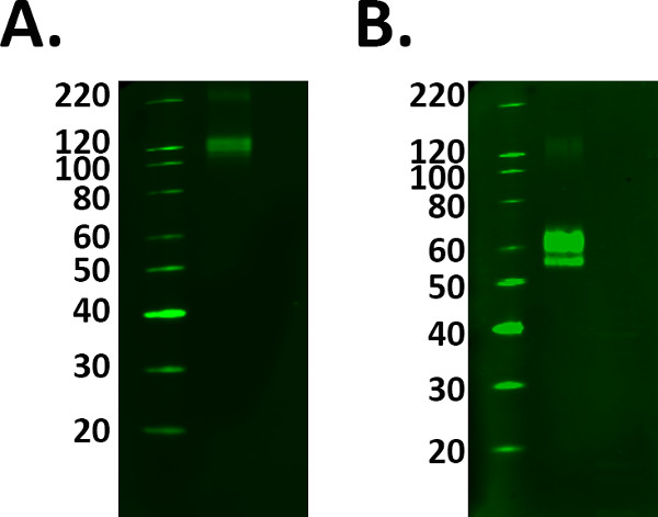
Figure 1. Positive control selection. The addition of positive controls to an experiment confirms the labeling detected is real. However, caution must be taken to ensure your control is working correctly prior to using experimental samples. A) Fusion protein TREM 2 was loaded at the manufacturer’s guidelines of 1 μg/ml, however the labeling observed at 110 kDa conflicts with the datasheet predicted molecular weight of 60-70 kDa. B) After addition and incubation with the reducing agent, the fusion protein labeling was detected at the predicted molecular weight. However, this meant a greater protein load was required as the reduction process decreased the signal of the protein.

2. Electrophoretic Separation of Proteins

1. Preparation of 4-12% Bis/tris gel (1.0 mm)
   NOTE: Gradient gels are used to produce greater protein separation across a broad molecular weight range.
   1. Select and prepare MES or MOPS running buffer (1 L per tank) by diluting with dH₂O. MES buffer produces better resolution of proteins within 3.5-160 kDa whereas MOPs running buffer is preferred to detect higher molecular weight proteins above 200 kDa however will have poorer resolution of lower molecular weight proteins below 15 kDa.
   2. Remove the comb and strip of tape that covers the foot of the gel. Gently wash the wells out with running buffer using a 1 ml pipette. Fill the wells with running buffer and ensure no bubbles remain in the gel. 
2. Gel preparation and loading
   1. Insert the gels into the tank and fill the inter gel compartment with running buffer to ensure all seals are working effectively.
   2. Add 3 μl of molecular weight standard into the first well in gel 1 and gel 2. Load 10 μl of each sample into subsequent wells.
      NOTE: With the exception of the ladders, gel 1 & gel 2 must be identical. It is imperative that the pre-stained molecular weight standard used for gel 2 is blue and visible when using a total protein stain in order to be visible in the 700 channel of Odyssey imager.
   3. Once both gels are loaded, fill the tank with the remaining running buffer and secure the lid.
3. Electrophoresis
   1. “Run” the gel at 80 V for 4 min to ensure the sample enters the polyacrylamide gel matrix in a uniform fashion. Thereafter increase the voltage and time to 180 V for 50 min respectively or until the sample dye can be seen at the foot of the gel.
      NOTE: Higher voltages can be applied to achieve shorter run times. However, this may result in “smiley” gels where the middle samples of the gels run faster than the outer lane samples caused by an increase in temperature¹⁴.

3. Total Protein Stain of the Loading Control Gel

1. Release gel 2 from the cassette using a gel knife. Remove the wells and the foot of the gel. Mark the gel to aid orientation.
2. Decant approximately 30 ml of the protein stain into a square Petri dish (approximate size 12 x 12 cm). Place gel 2 into the protein stain, ensuring the solution covers the entire gel, then agitate the gel for 1 hr minimum at room temperature to stain.
3. Decant the protein stain and wash the gel 3x in distilled water prior to visualization. Proceed to step 6.3 to visualize.

4. I-Blot Semi Dry Fast Protein Transfer

NOTE: All reagents required for protein transfer using the I-Blot machine are commercial products specifically designed for the I-Blot methodology and can be found in the Materials List.

1. Prepare the “bottom” transfer stack. Remove foil cover and pre-wet with running buffer direct from the gel tank. Pre-wet filter paper with distilled water.
2. Repeat step 3.1 and place gel 1 onto the prepared “bottom” transfer stack.
3. Lay the pre-wet filter paper over the gel. Roll the filter paper and gel to ensure no bubbles are trapped between the layers.
4. Remove the foil lid from the top transfer stack and lay the top stack on top of the filter paper and bottom stack. Roll the transfer stack “sandwich” to eliminate any air bubbles.
5. Insert the sponge from the transfer stack kit onto the lid of the I-Blot machine. Place the transfer stack sandwich onto the dedicated space on the I-Blot machine then close lid securely. Start the I-Blot and transfer for 8.5 min on program 3.
6. If there is a low protein signal or uneven high: low molecular weight protein ratios, test the manufacturer’s transfer times when using a semi dry “fast” transfer method. Run a simple optimization protocol using sample repeats of identical load to determine the ideal transfer voltage/time combination as seen in Figure 2.

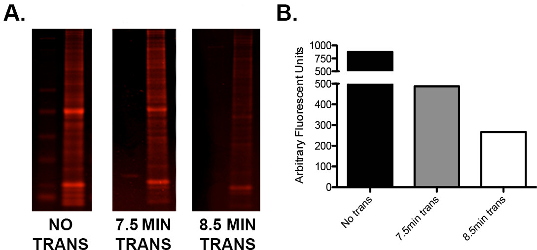
Figure 2. Optimization of transfer using the I-Blot. A) A single gel loaded with ladder and 15 μg of murine whole brain homogenate in three tandem repeats was cut into three sections. One section was not transferred, one was transferred for 7.5 min (as per manufacturer's guidelines) and one for 8.5 min. The gel sections were then stained with Instant Blue protein stain, scanned on an infrared imager in the 680 channel and quantified. B) Graphical representation of the quantification values demonstrating the difference in residual protein content of each gel following 0, 7.5, and 8.5 min of transfer. Note that an additional minute of transfer time resulted in additional protein transfer of approximately 45%. Please click here to view a larger version of this figure.

5. Antibody Detection of Proteins

1. Membrane preparation and blocking
   1. Remove transfer stack from the I-Blot machine. Remove the top and filter paper layer exposing the gel on the bottom transfer stack.
   2. Cut around the gel with a scalpel and ensure that a triangular cut for orientation purposes is represented on the membrane. Following membrane trimming, protein stain the gel to check transfer efficiency and/or discard.
   3. Swiftly move the membrane into a clean 50 ml tube (or equivalent receptacle) containing 5 ml of 1x PBS and place onto a mechanical roller (or orbital platform) for constant agitation.
      NOTE: It is critical that the membrane is not allowed to dry out. During semi-dry transfer the membrane will become hot. Wait 2 min before opening the transfer stack as this will allow it to cool and slow drying time during stack deconstruction. Use of a roller and tube for agitation during washes and incubations allows significant reduction in the volumes of solutions required.
   4. Wash the membrane 3 x 5 min in 1x PBS. Discard the 1x PBS and block the membrane with undiluted blocking buffer for a minimum of 30 min at room temperature.
2. Primary antibody preparation.
   1. Prepare the primary antibody according to the manufacturer's guidelines in 5 ml of blocking buffer with 0.1% Tween20. Incubate the membrane with the prepared primary antibody overnight at 4 °C with constant agitation.
      NOTE: Blocking buffer is generally used undiluted but may be diluted up to 1:4 with PBS if the primary antibody has high enough specificity.
   2. Discard the primary antibody and wash the membrane 6 times for 5 min each with 1x PBS.
3. Secondary antibody selection & preparation
   1. For secondary only labeling assessment for control purposes, omit steps 5.2.1 and 5.2.2 above and proceed to step 5.3 to determine sample specific secondary banding patterns. See Figure 3.

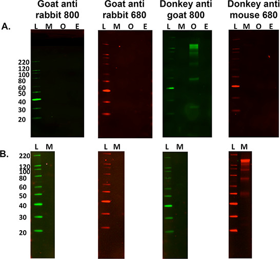
Figure 3. Optimization of secondary antibodies. A) A multi species comparison of secondary only non-specific labeling against 15 μg of murine (M), Ovine (O) and Equine (E) nervous tissue homogenates with a variety of fluorescent tagged secondary antibodies. L is the molecular weight ladder. Ovine tissue homogenate was the only sample to cross-react with the secondary labeling when using donkey anti-goat 800 antibody. B) It is also important to ascertain if non-specific labeling occurs when using a different tissue sample, i.e., murine gastrocnemius muscle (15 μg load). This sample cross reacts with the donkey anti-mouse 680 secondary antibody, however this did not occur when using mouse brain homogenate.

2. Prepare the fluorescent tagged secondary antibody 680 or 800 (red or green channel) following manufacturer recommended concentrations in blocking buffer with 0.1% Tween20. Incubate the membrane in the dark with the prepared secondary antibody for 90 min at room temperature with constant agitation.
3. Discard the secondary antibody and wash the membrane 6 times for 5 min per wash with 1x PBS. Proceed to step 6 — visualization.
   1. If visualization of markers is not working as expected, exam ladders with a range of secondary antibodies as a suitable additional step. Not all secondary antibodies allow visualization of all marker bands in all commercially available ladders.
   2. If expected bands are not visible, use an alternative secondary host, i.e., donkey anti rabbit versus goat anti rabbit represents a suitable protocol modification. See Figure 4. Host species used to raise a secondary antibody can occasionally cause an issue with visualization due to lack of specificity for specific primary antibodies. 

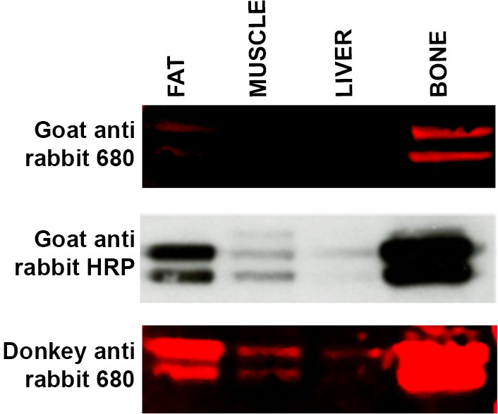
Figure 4. Troubleshooting secondary antibody specificity. Western blot of a range of tissue samples (15 μg protein per lane) — fat, muscle, liver and bone — incubated with ERK primary antibody and incubated with three different secondary antibodies. Top panel: WB labeled with LI-COR goat anti-rabbit 680 secondary antibody produced weak labeling of fat and bone and no signal was detected in the liver and muscle samples. Middle panel: Membrane (from top panel) was stripped and reprobed using ECL methodology and Goat anti-rabbit HRP linked secondary. Bands are now visible in muscle and liver samples and labeling appears more intense in the fat and bone samples. Bottom panel: Membrane (from top and middle panel) was stripped and reprobed using LI-COR Donkey anti-rabbit 680 secondary antibody which has shown a greater affinity for the ERK primary antibody. Labeling for muscle and liver is now visible with increased signal intensity from both fat and bone samples. Please click here to view a larger version of this figure.

6. Visualization

NOTE: All images are acquired using the LI-COR Odyssey Classic imager and associated Image Pro analysis software (version 3.1.4).

1. Turn and log on to the computer and imager. Open the imaging software and create a new file. See Figure 5.

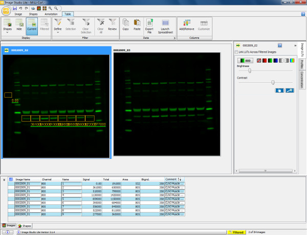
Figure 5. Visualization and quantification of western blot. Scan of a western blot showing murine gastrocnemius muscle (30 μg load) probed with Annexin V primary antibody (36 kDa) and goat anti-rabbit 800 secondary antibody. The membrane was scanned and visualized in the 800 channel. To quantify the protein (Annexin V), a rectangular box is drawn around the band of interest from sample 1. This is then copied and pasted over the remaining sample lanes to ensure measurement of the same area. Background is automatically accounted for around the shape drawn but this can be altered to ensure the background measurement is accurately defined. The table below displays the quantified measurements of each shape drawn including total signal obtained, background and signal with background subtracted. This information can then be exported into a spreadsheet program to calculate expression ratios (as determined by relative fluorescence intensity) and allows subsequent statistical analyses to be performed. Please click here to view a larger version of this figure.

2. Open the lid of the imager. Pour a small amount of 1x PBS on to the glass on the bottom left hand corner and then place the membrane on top of the PBS. Ensure the membrane is square with the axis on the imager and a 1 cm gap is left between the membrane and the grid axis.
   1. Roll the membrane to ensure no bubbles are trapped between the glass and the membrane.
   2. Count the number of squares the membrane occupies on the x and y axis. Close the lid of the imager. Enter the number of squares the membrane occupies on the computer software.
   3. Select the appropriate channel to scan the membrane which will depend on the fluorescent tag of the secondary antibody, i.e., 700 channel or 800 channel when a 680 or 800 fluorescent tagged antibody has been used respectively. When dual labeling is carried out, scan in both channels.
      NOTE: Optimize single protein labeling prior to carrying out dual labeling.
   4. Select the intensity to scan the membrane, if a high abundance protein use a low intensity scan. Alternatively if the primary antibody has poor affinity for the protein of interest select a higher intensity scan, i.e., level 5. Press start to begin the scan. Proceed to step 6.4.
3. Visualization of the loading control gel (Figure 6).
   
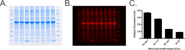
   Figure 6. Total protein labeling and analysis. A) Photograph of a total protein labeled gel containing 20 μg of equine cervical ganglia homogenate per lane. B) Gel from Panel A scanned in the 680 channel. C) Graph of quantified measurements from the total protein stained gel obtained using imaging software. A range of measurements determined by molecular weight markers, i.e., 30-110 kDa, are taken to provide a histogram of measurements to ensure standard error (SEM) is low (of the grouped samples) indicating that total protein levels in each sample are uniform across the gel. Please click here to view a larger version of this figure.
   1. Follow steps 6.1 and 6.2.
   2. Pour distilled water onto the glass in the bottom corner of the imager where the grid axis begins.
   3. Place the gel on top of the water and maneuver so the lanes are perpendicular to either the x or y axis of the grid. Leave a 1 cm gap between the y and x axis of the grid and the gel and count the number of squares the gel occupies on the grid axis. Close the lid of the imager.
   4. Enter the number of squares the gel occupies on the computer software.
   5. Select the 700 channel to scan the total protein stained gel.
      NOTE: Blue fluoresces in the 700 channel.
   6. Set the intensity to 5 and press start.
4. Quantification of scanned image
   1. Adjust the brightness and contrast buttons to produce the best image quality. If there appears to be high background noise, rescan the membrane at a lower intensity and use the high quality scan setting.
      NOTE: Any adjustments will not alter the fluorescent data acquired when scanning.
   2. Rotate images 90°, 180° and 270° in order to view in the desired orientation with no alteration to the data acquired. However, when making small adjustments of orientation in “free rotation”, by greater than 3°, data acquired in pixilation values can become distorted and thus affect the quantification results.
   3. Select a shape from the shapes menu — use a rectangle in most cases — and draw around the band of interest (WB) or the entire lane (total protein gel) in sample lane 1.
   4. Copy and paste the shape across to sample lane 2 band of interest or entire lane. Repeat across each individual band of interest for every sample and each lane for total protein gels.
   5. Check that the background measurement does not incorporate a signal in the next lane. The background can be automatically deducted by the software and encompass entire edge around the shape drawn or it can be specified to be top/bottom or left and right of the shape. Alternatively, designate a user defined background box.
   6. Display the signal for the shapes table for each shape drawn in arbitrary fluorescent units. The background will automatically be deducted from the signal.
   7. Export the image as a TIF file to view in different software. Do not export the image and manipulate using non image pro software as this will alter the original data acquired by the imager generating false data.
   8. Repeat steps 6.4.3-6.4.7 when quantifying dual labeling or carrying out multiple measurements on loading control gels to generate and collate standard error data. 

7. Post Visualization

1. Keep membranes in 1x PBS or dry out for long-term storage for future re-probing and stripping of membranes for other proteins of interest.
2. Stripping and re-probing of membranes. See Figure 7.
   
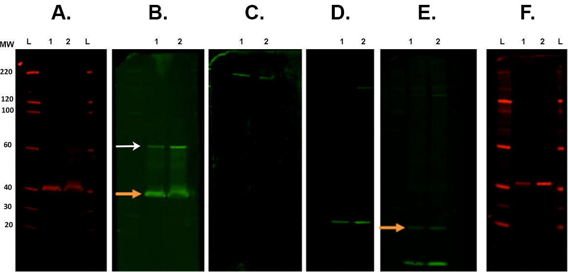
   Figure 7. Membrane stripping and reprobing. Representative examples of membranes following various stripping steps scanned with an infrared imaging system. A. The first immunodetection was carried out with CSP primary antibody (rabbit) and scanned at 700 channel. B. First stripping and reprobing with ROCK2 (rabbit) with 800 channel. Orange arrow indicates remaining CSP primary antibody present after the strip and re-probe. This does not affect the measurement of ROCK2 as the band is present at a higher molecular weight (white arrow). C. Second stripping and reprobed with β-Spectrin antibody (goat) and visualized in the 800 channel. D. Third stripping and reprobing with α-synuclein antibody (rabbit). E. Fourth stripping and reprobing with ubiquitin antibody (mouse) with 800 channel. There is still remaining signal from the last antibody (α-synuclein. Orange arrow). F. Fifth stripping and reprobing with CALB2 antibody (rabbit) imaged in 700 channel. Secondary antibodies used were: goat anti-mouse 800cw, goat anti-rabbit 680rd, goat anti-rabbit 800cw, donkey anti-goat 800cw (see Materials List). Lane labels: L — ladder, 1/2 — sample 1/2. Please click here to view a larger version of this figure.
   1. Place membrane(s) in a square Petri dish that contain approximately 30 ml of Revitablot stripping buffer and are incubated between 5-20 min at room temperature with constant agitation.
   2. Wash the membrane(s) 3 times in PBS then rescan on the imager to ensure complete removal of fluorescence has occurred — this step should be repeated after every strip.
   3. Incubate membrane(s) for longer periods if fluorescence remains. Rescan the membrane after each strip to confirm that there is no secondary signal remaining.
      NOTE: Membrane(s) should only be stripped and reprobed a maximum of 3 times in order to guarantee that the integrity of the membrane has not been compromised resulting in undesirable high background to signal ratio.