Learning Objectives

The raw data from most DSC experiments are presented as a heat flux versus temperature graph, as the calorimeter actually measures the difference in the rate of heat flow into the sample solution and buffer ³⁵. Therefore, if both cells (i.e. sample and reference cells) contain identical solutions during an experiment, the raw data from the scan should be a flat line with no observable peaks. Any peak observed can be attributed to instrumentation error (e.g. damaged or contaminated cells), which is why running buffer scans prior to sample analysis is an adequate system suitability test. Figure 1 illustrates the result of a typical buffer scan indicating that the calorimeter was in good working condition prior to sample analysis.

Figure 2 shows the raw data for a DSC experiment carried out on different lots of two protein samples. As implied earlier, the observed peaks are the differences in the heat flux of the samples and their respective buffers. Differences in sample concentration can cause variations in heat capacity recorded by the calorimeter; however, these variations are normalized during sample analysis as per section 4.2 of the procedure. Higher concentrations can also reveal additional thermodynamic domains not contributing to the transition at lower concentrations. In addition, each transition represents a thermodynamic domain that may include one or more structural domains of the protein ³⁶. In this case, the Protein 1 has three structural domains that melt cooperatively.

Figure 3 shows the results generated from the analysis of the raw data for protein 1 and 2 presented in Figure 2, i.e., after baseline subtraction and iterative curve fitting. The resulting thermograms have been normalized for scanning rate (automatically carried out by a pre-set algorithm in the analysis software) and concentration; thus, presenting the results of the experiment in comparable heat capacity versus temperature graphs. The analysis software uses data from the Heat Capacity versus Temperature graphs, such as T_m and ΔCp, to derive other thermodynamic parameters using variations of the equations given above depending on the cooperativity of protein unfolding.

When testing unknown samples, setting the appropriate temperature range is crucial. Otherwise, incomplete thermograms may result, as illustrated in Figure 4. Although T_m from such profiles can be derived, ΔH cannot be accurately determined. Therefore, the sample must be retested with a larger temperature range to completely capture the thermal transition. Some proteins also readily form aggregates after complete denaturation, resulting in an increasing post-transition heat capacity: this often appears as an incomplete thermogram as illustrated in Figure 2B. However, retesting with a higher final temperature can help confirm whether there is an occurrence of a conformational transition at that region of the thermogram or it is merely the heat absorbing effect of protein aggregates.

Thermal stability is one of the most significant physical properties of proteins and protein-based products in the industry ³⁷. In pharmaceuticals, it is used to determine the stability of biologics under different conditions, including formulation buffers and environmental factors such as humidity and temperature. It is also used to monitor key manufacturing step (e.g., purification and detoxification) to ensure conformational consistency between production lots. Figures 5 and 6 illustrate the use of DSC to examine the effects of chemical detoxification and storage conditions respectively on the stability and structural conformation of two different proteins. The significant differences in Tm and ∆H indicate conformational changes and protein degradation respectively. In addition, the loss of the third transition in Figure 6 further illustrates the degradation of a domain which was confirmed by a decrease in molecular weight when the samples were analyzed using Size-Exclusion Chromatography with multi-angle light scattering (SEC-MALS) (data not shown).

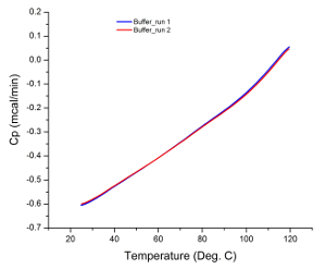
Figure 1: Buffer Scans. The similarity in gradient of each scan with no observable peaks indicates that the instrument is in good working condition and generated reproducible results. Please click here to view a larger version of this figure.

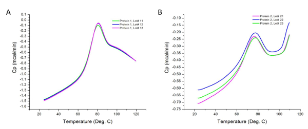
Figure 2: Raw Data Collected from DSC Experiments. These graphs are good representations of the unanalyzed (raw) data acquired after experimental runs (i.e. prior to baseline subtraction and curve fitting). Each line represents a production lot. Protein 2 tends to aggregate more readily upon heating, resulting in an increase in heat capacity above 100 °C in the post-transition region of the thermogram. Please click here to view a larger version of this figure.

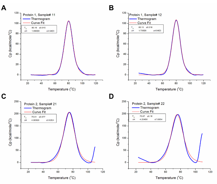
Figure 3: Analyzed DSC Data. These graphs are good representations of analyzed DSC data (i.e. after baseline subtraction and curve fitting). The blue line represents the thermogram after baseline subtraction, while the red line represents the curve with the best fit to the thermogram. (A) The T_m and ΔH for Protein 1 Sample # 12 are 80.16 °C and 1.69 x 10⁶ cal/mol respectively. (B) The T_m and ΔH for Protein 1 Sample# 13 are 80.15 °C and 1.71 x 10⁶ cal/mol respectively. (C) The T_m and ΔH for Protein 2 Sample # 21 are 75.01 °C and 4.08 x 10⁶ cal/mol respectively. (D) The T_m and ΔH for Protein 2 Sample # 22 are 75.67 °C and 4.22 x 10⁶ cal/mol respectively. Please click here to view a larger version of this figure.

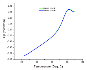
Figure 4: An Incomplete Thermogram. Raw data collect for Protein 1 analyzed at an inadequate temperature range. The final temperature of experiment was set to 90 °C which did not accommodate the entire transition profile of the protein as compared to the experiment for Figure 2A which was set to 120 °C. Please click here to view a larger version of this figure.

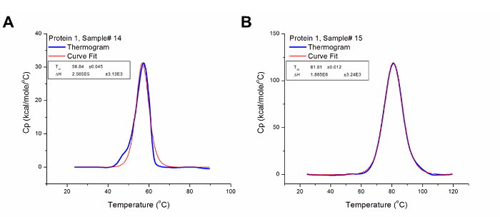
Figure 5: Analyzed Data Showing the Effect of Chemical Detoxification on the Tertiary Structure of Protein 1. (A) Protein 1 is a toxin in its native conformation and has its T_m at 56.84 °C and ΔH at 2.57 x 10⁵ cal/mol. (B) The detoxified form of Protein 1 (i.e. toxoid) has T_m and ΔH values of 81.01 °C and 1.89 x 10⁶ cal/mol respectively. Thus, it can be concluded that the detoxification step introduced some form of variation to the structural conformation of Protein 1 which confers greater stability (higher T_m) to its detoxified form. Please click here to view a larger version of this figure.

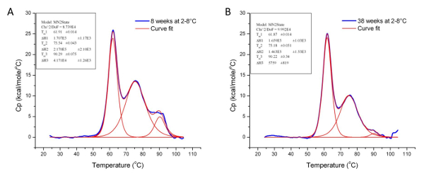
Figure 6: Analyzed Data Showing the Effect of Storage Conditions on the Conformation of Protein 3. These graphs illustrate the effect of storage temperature (2 – 8 °C) on the stability and tertiary structure of Protein 3 over 30 weeks. The T_m and ΔH values for Protein 3 at the 8^th (A) and 38^th week (B) of storage are given in Table 1 below. Please click here to view a larger version of this figure.

Table 1: Tm and ΔH Values for Protein 3 at the 8^th and 38^th Week of storage at 2 – 8 °C. Although the T_m values at both time points are similar, the difference in the ΔH values indicates that the tertiary structure of Protein 3 has degraded over 30 weeks under the specified storage condition.