Science Education
>

How to Find Effects of Stimulus Processing on Event Related Brain Potentials of Close Others when Hyperscanning Partners

Instructor Prep
concepts
Student Protocol
JoVE Journal
Neuroscience
This content is Free Access.
JoVE Journal Neuroscience
How to Find Effects of Stimulus Processing on Event Related Brain Potentials of Close Others when Hyperscanning Partners

All methods described herein were pre-approved by the Douglas Institute Research and Ethics Board.

1. Participant recruitment, in-lab greeting and questionnaires

  1. Recruit pairs of participants (close friends/siblings/spouses ages 18-35) and inform them they will have to separately complete a Friendship Eligibility Questionnaire upon arrival in the lab to ensure only close others are included in the experiment[see Annex 1 for an example advertisement].
  2. Make sure they meet all the other inclusion criteria (i.e. right-handedness, university level education, perfect or corrected to perfect vision, no contact lenses, no dreads, no drug abuse, no psychiatric disorder, no use or psychotropic medications). Schedule their visit to the lab if they are eligible.
  3. Greet the pair of participants upon their arrival at the lab. Obtain informed consent, separate them and have each participant fill out the Friendship Eligibility Questionnaire and McGill Friendship Questionnaire alone.
  4. This is used to assess their attitude about their relationship and to exclude partners who are not close enough and do not reach the minimum score of 13 correct answers.
  5. Once their answers have been sent to the lab's database, check for at least 13 correct answers from each participant.
  6. Escort the partners into the EEG recording rooms. Turn on the stimulus presentation computer and the EEG acquisition computer. Start the EEG acquisition application [Photo 1] and set the status of the EEG channels to " impedance check" [Photo 2].
  7. Have each participant sit at a designated computer desk in the adjacent rooms separated by a glass window. Keep the curtains open so that each participant can see his or her partner. Encourage them to talk (e.g., about their answers at the Friendship Eligibility Questionnaire) in order to maintain the feeling of the presence of the other.

2. Electrode cap placement (see Gu et al., 2014)

  1. Measure the size of the head of the participant and use the pencil to mark Fp1 and Fp2 electrode sites and select the cap of appropriate size.
  2. Clean the forehead and earlobes of each participant with an alcohol swab.
  3. Insert two frontal sticky sponge discs in the EEG electrode cap on Fp1 and Fp2.
  4. Place the sticky ends of the discs against the forehead of the participant at the marked Fp1 and Fp2 locations. Ask the participant to press them firmly and pull the cap over the head to snugly fit the cranium. Check whether the cap is fitted symmetrically over the head (both from right vs. left and forward vs. backward perspectives) and then connect the EEG outlet to the amplifier's plug.
  5. Using a 10mL blunt needle tip syringe, gently but firmly touch the scalp of the participant and move the needle sideways to tease the hair apart. Insert conductive gel (~0.5mL) from that position on the scalp and up to create a column of gel in the ground electrode first. Then, insert gel into both ear electrodes and attach them to the earlobes. Plug the left ear electrode into the top channel and the right one, which will be used as the reference, below it in its amplifier box.
  6. Using a sterilized blunt needle tip previously fitted to the syringe, move the hair strands apart by wiggling the syringe in all the other electrode sites, ensuring that the tip is in contact with the scalp. Then, start inserting conductive gel in each of the other electrode placements with a slow upward motion in order to build a column of gel that will go from the scalp to the metal of the electrode.
  7. Use a sterile sharp needle to cautiously and gently scratch the surface of the scalp through each electrode, starting with the ground and the ears, to remove dead skin and increase electrical conductance by having the gel make contact with the living cells of the scalp and earlobes.
  8. Check for proper impedance while scratching the scalp. The lights corresponding to the electrode channels on the amplifier boxes will change color from orange to green as the impedance for each channel drops below 5 kΩ [see Photo 3].
    1. Note: if a particular electrode is not functioning properly, add more gel and scratch a bit more with the needle. If the problem persists, use a shortcut wire by plugging it inside the slot for the faulty electrode on the amplifiers and hooking up the other end to the electrode placement in the EEG cap.

3. EEG/ERP data recording 4. EEG/ERP data recording

  1. Just prior to the experiment, instruct the participants to try to feel the presence of their partner during the entire testing period. Then, draw the curtains on both sides of the double-glass window, dim the lights, and close the door of each participant's room.
  2. Type in the appropriate command for the given stimulus sequence in order to run the stimulus presentation software. Then, start recording the EEG of both participants while they are presented with the visual stimuli simultaneously.
  3. Once the stimulus presentation sequence is complete, stop recording the EEG data.
  4. At the end of the experiment, carefully remove the EEG caps and assist the participants in washing and drying their hair.
  5. After the participants have cleaned their hair, have them complete a debriefing questionnaire in which they report the degree to which they felt the presence of their partner, specifically during which part of the experiment and for how long they felt this way.
  6. Detach the cap and ear electrodes from the amplifiers, remove the disposable sponge discs, and clean the cap and ear electrodes under running water. Use a mild soap and a toothpick to clear the gel from the electrodes, Rinse thoroughly and allow the EEG cap to air dry.
  7. Save the recorded data on USB drive by inserting the USB drive into one of the USB ports on the EEG data acquisition computer and dragging the data file into the USB directory. Then, transfer the data to another computer for data processing.

4. Data processing

Note: all data processing is done using EEGLab.15

  1. Open the data processing software [see Table of Materials] and then, EEGLab by typing "eeglab" in the command interface [see Screenshot 1 & 2].
  2. Import the data file. For this step, first, click "File" on the EEGLAB GUI, select "Import data", select "Using EEGLAB functions and plugins", and click "From EDF/EDF+/GDF files (BIOSIG toolbox)" [see Screenshot 3]. Choose the desired data file.
  3. Create and EEG event list, which consists of a list of entries that correspond to the difference types of visual stimuli that were used during experiment (i.e. the same image believed to be different labeled "S-BD" and the different image believed to be different labeled "D-BD"). To do this, click on "ERPLAB" on the EEGLAB GUI, select "EventList," and click "Create EEG EVENTLIST" [see Screenshot 4]. In the new window, enter the relevant information under "Event info" and "Bin info (optional)" for the S-BD category and click "Update Line". Repeat this process for the D-BD category. Click "APPLY" [see Screenshot 5].
  4. Extract the bin-based epochs, each epoch (or trial) consisting of a single ERP waveform that spans 1,204 ms from -204ms to 1000ms, where 0 corresponds to the onset of the visual stimulus. For this step, select "ERPLAB" on the EEGLAB GUI and click "Extract bin-based epochs" [see Screenshot 6]. In the new window under "Bin-based epoch time range (ms)," write "-204 -4". Click "RUN" [see Screenshot 7].
  5. Perform artifact detection on the epochs. This step removes all the trials that have altered been by amplifier saturation or A/D clipping. Epochs with segments that are inferior to -100 microvolts and/or superior to +100 microvolts will be eliminated for the 4 frontal EEG electrodes (Fp1, Fp2, F7, and F8). Similarly, epochs with segments that are inferior to -75 microvolts and/or superior to +75 microvolts will be deleted for the remaining 24 non-frontal electrodes. Additionally, epochs containing segments that include flat lines that persist for more than 100ms will be cut out in all 28 electrodes. To eliminate the extreme voltages, first click "ERPLAB" on the EEGLAB GUI, then select "Artifact detection in epoched data" and click "Simple voltage threshold" [see Screenshot 8]. In the new window under "Test period (start end) [ms]," write "-204 1000"; under "Voltage limits[uV] (e.g. -100 100):" write "-100 100"; under "Channel(s)," write "1:4" (to select only the 4 frontal electrodes). Select "ACCEPT" [see Screenshot 9]. Repeat this process for the remaining 24 electrodes, making the appropriate changes where necessary (i.e. writing "-75 75" instead of "-100 100" for the voltage limits; writing "5:28" instead of "1:4" to select the remaining 24 electrodes). Next, to remove the flat lines, click "ERPLAB" on the EEGLAB GUI, select "Artifact detection in epoched data", and click "Blocking & flat line" [see Screenshot 10]. In the new window under "Test period (start end) [ms]", write "-204 1000"; under "Amplitude tolerance (single value, e.g. 2):", write "-1e-07 1e- 07"; under "Duration [ms]", write "100"; under "Channel(s)", write "1:28" (to select all 28 electrodes). Select "ACCEPT" [see Screenshot 11].
  6. Compute the averaged ERPs of each participant for each condition (consistent vs. inconsistent). To do this, click "ERPLAB" on the EEGLAB GUI and select "Compute averaged ERPs" [see Screenshot 12].
  7. Compute the grand averages for the ERP sets in each condition (consistent vs. inconsistent) and plot the resulting ERP waveforms. For this step, click "ERPLAB" on the EEGLAB GUI and select "Average across ERPsets (Grand Average)" [see Screenshot 13]. In the new window, add the relevant ERP sets by clicking "Add Erpset" and then, click "RUN" [see Screenshot 14]. To plot the ERP waveforms, click "ERPLAB" on the EEGLAB GUI, click "Plot ERP", and select "Plot ERP waveforms" [see Screenshot 15]. In the new window under "Time range (min max, in ms)", write "-204.0 1000.0" and click the button "positive is up" (this will change the label of the button to "negative is up" so that negative y-values are displayed above the x-axis); under "Style", select "Topographic" and change the "w" and "h" values to "0.1". Click "PLOT" [see Screenshot 16].

How to Find Effects of Stimulus Processing on Event Related Brain Potentials of Close Others when Hyperscanning Partners

Learning Objectives

Three figures have been presented herein. Each part of these figures (28 parts in total) represents a single EEG channel with its own label (i.e. Fp1, Fp2, F7, F8, etc.). Figure 1 shows a typical example of "good" results, depicting ERP waveforms obtained from a single participant. The black lines correspond to the consistent condition and the red lines correspond to the inconsistent condition. In contrast, Figure 2 depicts "poor" results due to a problematic session for which the waveforms portray either unintelligible ERP components, flat lining, or noise. These were also obtained from one participant. The black lines correspond to the consistent condition and the red lines correspond to inconsistent condition. Figure 3 shows a grand average of 27 ERP sets from the participants who felt together during more than 50% of the experiment. The black lines correspond to the control-consistent category and the red lines correspond to the critical-inconsistent category. Figure 4 is a depiction of the average of ERP's from the 13 individuals who felt together for more than 50% of the trials and for whom the inconsistent condition was more positive at the F8 electrode site for the 75-150ms time window. The inconsistent condition is more positive than the consistent condition for most electrodes.

Figure 1
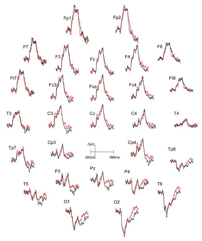
Figure 1: Typical "good" results representing ERPs from one participant. Each part (28 parts in total) represents a single EEG channel with its own label (i.e. Fp1, Fp2, F7, F8, etc.). The ERP components are well defined in the waveforms. The black lines correspond to the consistent condition (different stimulus condition, or DSC) and the red lines correspond to the inconsistent condition (identical stimulus condition, or ISC). Please click here to view a larger version of this figure.

Figure 2
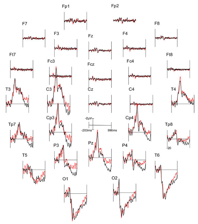
Figure 2: Typical "Poor" results representing ERPs from one participant. Each part (28 parts in total) represents a single EEG channel with its own label (i.e. Fp1, Fp2, F7, F8, etc.). The black lines correspond to the consistent condition (DSC) and the red lines correspond to inconsistent condition (ISC).
The ERP components are not well defined in the waveforms and many are marked by a flat-line (i.e. F8, Fc4). Please click here to view a larger version of this figure.

Figure 3
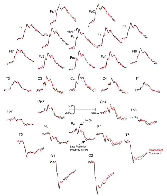
Figure 3: Grand averages of ERPs of the 27 participants who felt together. 
Each part (28 parts in total) represents a single EEG channel with its own label (i.e. Fp1, Fp2, F7, F8, etc.). The black lines correspond to the consistent condition (DSC) and the red lines correspond to the inconsistent condition (ISC). Please click here to view a larger version of this figure.

Figure 4
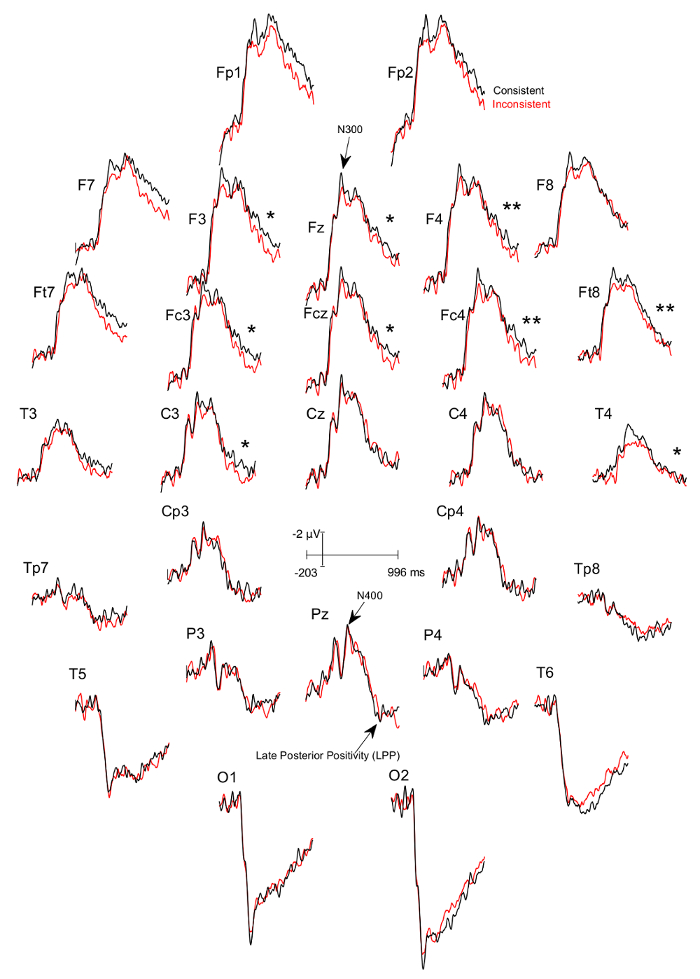
Figure 4: Grand averages of ERPs of the 13 participants who felt together and for whom the ERPs to the consistent DSC-trials was more negative at the F8 electrode site between 75-150ms than the ERPs to the inconsistent ISC-trials. Each part (28 parts in total) represents a single EEG channel with its own label (i.e. Fp1, Fp2, F7, F8, etc.). The black lines correspond to the consistent condition and the red lines correspond to the inconsistent condition. There is a significant difference in the 600 – 900 ms time window between the consistent and inconsistent condition at F3 (p=0.024), F4 (p=0.001), Fz (p=0.024), Fc3 (p=0.041), Fcz (p=0.022), Fc4 (p=0.002), Ft8 (p=0.004), C3 (p=0.022), and T4 (p=0.039), with the inconsistent condition being more positive. Please click here to view a larger version of this figure.

Supplemental File 1 Please click here to download this file.

Supplemental File 2 Please click here to download this file.

Supplemental File 3 Please click here to download this file.

Supplemental File 4 Please click here to download this file.

List of Materials

EEG acquisition software Psychlab http://www.psychlab.com/softw_general.html
8 Digital EEG Amplifiers (NuAmp) Neuro Scan Labs
2 computers
Matlab The MathWorks, Inc http://www.mathworks.com/products/matlab/
EEGLab Matlab toolbox http://sccn.ucsd.edu/eeglab/
ERPLAB Toolbox http://erpinfo.org/erplab
Stimulus generation software E-Prime
ECI Electrode cap Electro-cap International, Inc http://www.electro-cap.com/index.cfm/caps/
Special Head Measuring Tape (4 Color ribbon) Electro-cap International, Inc http://www.electro-cap.com/index.cfm/supplies/
Disposable Sponge Disks Electro-cap International, Inc http://www.electro-cap.com/index.cfm/supplies/
Cap straps Electro-cap International, Inc http://www.electro-cap.com/index.cfm/supplies/
Electro-gel Electro-cap International, Inc http://www.electro-cap.com/index.cfm/supplies/
Blunt needle (BD Vacutainer PrecisionGlide Multiple Sample Needle) Becton, Dickinson and Company
2 Syringes Electro-cap International, Inc http://www.electro-cap.com/index.cfm/supplies/
4 Ear Electrodes Electro-cap International, Inc http://www.electro-cap.com/index.cfm/supplies/
Alcohol wipes
2 Red pencils
Facilities and supplies for participants to wash their hair after the experiment- sink, shampoo, comb, towels, hair dryer

Lab Prep

The partners of each pair must be able to pass the McGill Friendship Questionnaire without communicating. Each partner is then seated in front of a screen in one of two adjacent rooms. These rooms are separated by a glass window through which participants communicate to maintain feelings of togetherness while being fitted with the EEG cap. After checking for adequate EEG signals, the glass is covered by a curtain to prevent visual communication. Then, partners must be silent but are instructed to try to feel in the presence of their partner during the entire experiment. Just before it starts, participants are told that each of them will be presented with one image at a time and that these images will occur at the same time for both of them on their own screen. They are also instructed that, for each trial, the simultaneous images will always be different. However, unbeknownst to them, trials are randomized: only half of them are consistent with this instruction and actually include two different images. These trials form the DSC, that is, the different-stimuli condition. The other half of the trials are inconsistent with the instruction. They include two identical images and form the ISC (identical-stimuli condition). After the experiment, participants are sorted into two groups: those who reported that they felt in the presence of their partner during the majority of the trials and those who reported they did not. The impact of the stimulus processing of the partner is found by subtracting the mean voltages of the ERPs of the ISC (inconsistent with the instructions) from the ERPs of the DSC (consistent with the instructions) in at least two time windows (TWs): firstly, in the 75 to 150 ms TW, where the absolute values of these subtractions are greater, especially at right frontal sites, in those who felt in the presence of their partner than in those who did not; secondly, in the LPP time window (i.e., from 650 to 950 ms post onset), where ERPs are significantly less positive in the DSC than in the ISC in those in whom the raw results of the early (75-150ms) subtractions are negative.

The partners of each pair must be able to pass the McGill Friendship Questionnaire without communicating. Each partner is then seated in front of a screen in one of two adjacent rooms. These rooms are separated by a glass window through which participants communicate to maintain feelings of togetherness while being fitted with the EEG cap. After checking for adequate EEG signals, the glass is covered by a curtain to prevent visual communication. Then, partners must be silent but are instructed to try to feel in the presence of their partner during the entire experiment. Just before it starts, participants are told that each of them will be presented with one image at a time and that these images will occur at the same time for both of them on their own screen. They are also instructed that, for each trial, the simultaneous images will always be different. However, unbeknownst to them, trials are randomized: only half of them are consistent with this instruction and actually include two different images. These trials form the DSC, that is, the different-stimuli condition. The other half of the trials are inconsistent with the instruction. They include two identical images and form the ISC (identical-stimuli condition). After the experiment, participants are sorted into two groups: those who reported that they felt in the presence of their partner during the majority of the trials and those who reported they did not. The impact of the stimulus processing of the partner is found by subtracting the mean voltages of the ERPs of the ISC (inconsistent with the instructions) from the ERPs of the DSC (consistent with the instructions) in at least two time windows (TWs): firstly, in the 75 to 150 ms TW, where the absolute values of these subtractions are greater, especially at right frontal sites, in those who felt in the presence of their partner than in those who did not; secondly, in the LPP time window (i.e., from 650 to 950 ms post onset), where ERPs are significantly less positive in the DSC than in the ISC in those in whom the raw results of the early (75-150ms) subtractions are negative.

Procedure

The partners of each pair must be able to pass the McGill Friendship Questionnaire without communicating. Each partner is then seated in front of a screen in one of two adjacent rooms. These rooms are separated by a glass window through which participants communicate to maintain feelings of togetherness while being fitted with the EEG cap. After checking for adequate EEG signals, the glass is covered by a curtain to prevent visual communication. Then, partners must be silent but are instructed to try to feel in the presence of their partner during the entire experiment. Just before it starts, participants are told that each of them will be presented with one image at a time and that these images will occur at the same time for both of them on their own screen. They are also instructed that, for each trial, the simultaneous images will always be different. However, unbeknownst to them, trials are randomized: only half of them are consistent with this instruction and actually include two different images. These trials form the DSC, that is, the different-stimuli condition. The other half of the trials are inconsistent with the instruction. They include two identical images and form the ISC (identical-stimuli condition). After the experiment, participants are sorted into two groups: those who reported that they felt in the presence of their partner during the majority of the trials and those who reported they did not. The impact of the stimulus processing of the partner is found by subtracting the mean voltages of the ERPs of the ISC (inconsistent with the instructions) from the ERPs of the DSC (consistent with the instructions) in at least two time windows (TWs): firstly, in the 75 to 150 ms TW, where the absolute values of these subtractions are greater, especially at right frontal sites, in those who felt in the presence of their partner than in those who did not; secondly, in the LPP time window (i.e., from 650 to 950 ms post onset), where ERPs are significantly less positive in the DSC than in the ISC in those in whom the raw results of the early (75-150ms) subtractions are negative.

Tags