Representative staining patterns of different markers can be seen in Figure 1. The pattern varies depending on the distribution of the protein. Examples of five rostro-caudal levels are shown in columns (A)-(E). A representative DAPI staining is shown in the first row: DAPI adheres to the DNA of a cell and thus nuclei are stained. This results in a punctate pattern. Regions with a high cell density are brighter than regions with low cell densities. An example for a heterogeneously distributed protein can be seen in the second row. The Mover staining reveals a differential distribution throughout the brain, with bright hotspot areas and dimmer areas. In the third row, an example for the more homogeneously distributed reference marker synaptophysin is shown. An overlay of the two proteins (fourth row) shows the differential distribution of Mover (red) compared to the marker protein synaptophysin (green).
Figure 2 shows the quantification described in step 4 of the protocol. Shown are the mean fluorescence intensity values for the different channels across the hemispheres (Mover, Figure 2A; synaptophysin, Figure 2B) and across the areas of interest (Mover, Figure 2C; synaptophysin, Figure 2D). To determine the Mover abundance relative to the number of synaptic vesicles, a ratio is taken of the Mover fluorescence values to synaptophysin fluorescence values. These ratios for the areas of interest are shown in Figure 2E, and already provide an indication of the heterogeneous distribution of Mover, with areas with high and low Mover levels relative to synaptic vesicles. To additionally compensate for the inherent technical variability, the ratio in one area of interest (Figure 2E) is compared to that across the hemisphere (not shown) and translated into a percentage. This relative Mover abundance (Figure 2F) gives a measure of how much Mover is present in one area of interest relative to average.
As mentioned above, one of the major advantages of this technique is the ability to determine the abundance of the protein of interest across very small areas, even subregions and layers of areas of interest. One example of this application is shown in Figure 3, where the relative Mover abundance was determined for the different layers in the subfields of the hippocampus. The quantification in the different layers shown in Figure 3D, Figure 3F, and Figure 3H corresponds to the layers shown in Figure 3C, Figure 3E, and Figure 3G, with the corresponding colors. Within the hippocampus, Mover is heterogeneously distributed, with high Mover levels relative to synaptic vesicles in layers associated with intra-hippocampal computation (i.e., the polymorph layer of dentate gyrus [DG], stratum radiatum, lucidum and oriens of Cornu Ammonis 3 [CA3], and stratum radiatum and oriens of Cornu Ammonis 1 [CA1]), and low levels in input- and output layers (the inner and outer molecular layer of DG, the pyramidal cell layers of CA3 and CA1, and the stratum lacunosum-moleculare of CA1).
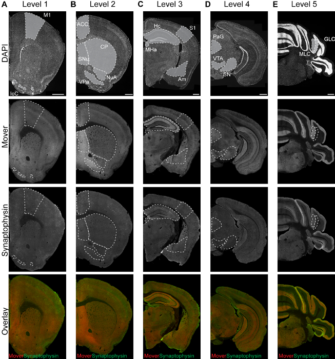
Figure 1: Representative immunofluorescence images of DAPI (first row), Mover (second row), synaptophysin (third row), and their overlay (fourth row, Mover in red, synaptophysin in green) at the 5 rostro-caudal levels (A-E). Areas of interest are shaded in grey in the upper row of panels. M1, primary motor cortex; IoC, islands of Calleja; ACC, anterior cingulate cortex; SNu, septal nuclei; VPa, ventral pallidum; NuA, nucleus accumbens; CP, caudate putamen; S1, primary somatosensory cortex; Hc, hippocampus; Am, amygdala; MHa, medial habenula; PAG, periaqueductal grey; SN, substantia nigra; VTA, ventral tegmental area; MLC, molecular layer of the cerebellum; GLC, granular layer of the cerebellum. Scale bar = 500 µm. This figure has been modified from Wallrafen and Dresbach1. Please click here to view a larger version of this figure.
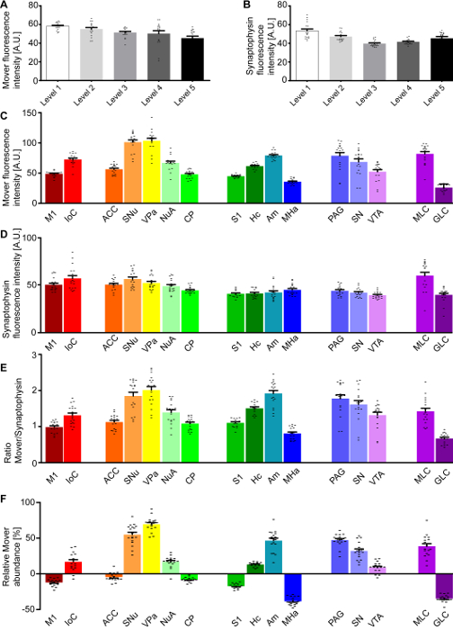
Figure 2: Quantification of the Mover distribution across the 5 rostro-caudal levels. Mean fluorescence intensity of the Mover signal (A) and the synaptophysin signal (B) at the different levels. Mean fluorescence intensity of the Mover signal (C) and the synaptophysin signal (D) at the 16 manually delineated brain regions. (E) Ratios of Mover and synaptophysin in the 16 brain areas of interest. (F) Quantification of the relative Mover abundance, comparing Mover/synaptophysin ratio at the respective region to the ratio of the corresponding hemisphere. M1, primary motor cortex; IoC, islands of Calleja; ACC, anterior cingulate cortex; SNu, septal nuclei; VPa, ventral pallidum; NuA, nucleus accumbens; CP, caudate putamen; S1, primary somatosensory cortex; Hc, hippocampus; Am, amygdala; MHa, medial habenula; PAG, periaqueductal grey; SN, substantia nigra; VTA, ventral tegmental area; MLC, molecular layer of the cerebellum. Black dots represent single data points. Bars show the mean ± standard error of the mean (SEM). This figure has been modified from Wallrafen and Dresbach1. Please click here to view a larger version of this figure.
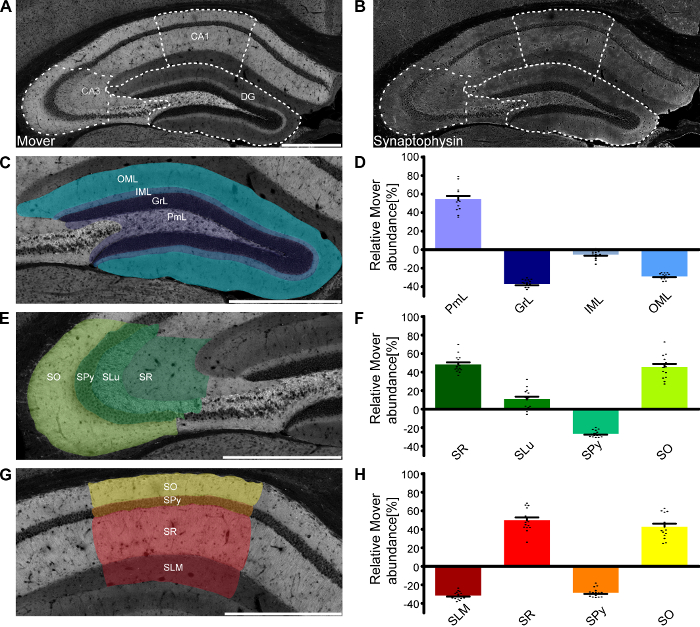
Figure 3: Mover distribution in the mouse hippocampus. Immunofluorescence stainings of coronal slices of the mouse hippocampus. Overview of the hippocampus showing the heterogeneous Mover expression pattern (A) and the corresponding Synaptophysin staining (B). The three regions of interest (DG, Figure 3C; CA3, Figure 3E; CA1, Figure 3G) are delineated with white dotted lines. (D,F,H) Quantification comparing the ratio in the respective layers to the ratio of the corresponding hemisphere. The colors in the bar graphs correspond to the respective shading in panels C, E, and G. Mover expression is high in levels associated with intra-hippocampal computation (i.e., the polymorph layer of DG, stratum radiatum, lucidum and oriens of CA3, and stratum radiatum and oriens of CA1), and low in the main input- and output layers (the inner and outer molecular layer of DG, the pyramidal cell layers of CA3 and CA1, and the stratum lacunosum-moleculare of CA1). OML, outer molecular layer; IML, inner molecular layer; GrL, granular layer; PmL, polymorph layer/hilus; SO, stratum oriens; SPy, stratum pyramidale; SLu, stratum lucidum; SR, stratum radiatum; SLM, stratum lacunosum-moleculare. Scale bar = 500 µm. Black dots represent single data points. Bars show the mean ± SEM. This figure has been modified from Wallrafen and Dresbach1. Please click here to view a larger version of this figure.
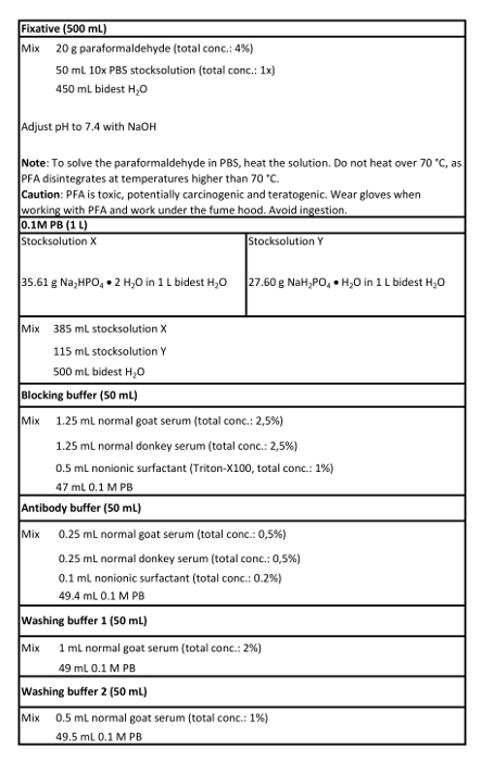
Table 1: Solutions used in this protocol.
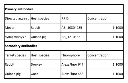
Table 2: Antibodies used in this protocol.
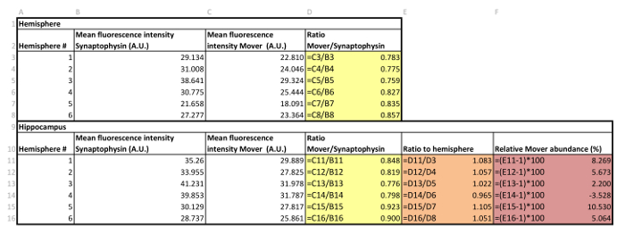
Table 3: Example of data handling.