1. Design the FRET assay.
- Download the structure file of the Cul1•Cand1 complex from the Protein Data Bank (file 1U6G).
- View the structure of the Cul1•Cand1 complex in PyMOL.
- Use the Measurement function under the Wizard menu of PyMOL to estimate the distance between the first amino acid of Cand1 and the last amino acid of Cul1 (Figure 1).
- Load the online spectra viewer (see Table of Materials) and view the excitation and emission spectra of 7-amino-4-methylcoumarin (AMC) and FlAsH simultaneously (Figure 2). Note that AMC is the FRET donor and FlAsH is the FRET acceptor.
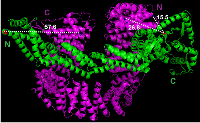
Figure 1: The crystal structure of Cul1•Cand1 and measurement of the distance between potential labeling sites. The crystal structure file was downloaded from Protein Data Bank (File 1U6G), and viewed in PyMOL. Measurements between selected atoms were done by PyMOL. Please click here to view a larger version of this figure.
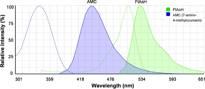
Figure 2: The excitation and emission spectra of the fluorescent dyes for FRET. Spectra of AMC (7-amino-4-methylcoumarin) and FlAsH are shown. Dashed lines indicate excitation spectra, and solid lines indicate emission spectra. The image was originally generated by the Fluorescence SpectraViewer and was modified for better clarity. Please click here to view a larger version of this figure.
2. Preparation of Cul1AMC•Rbx1, the FRET donor protein
- Construct plasmids for expressing human Cul1sortase•Rbx1 in E. coli cells. Note that the two plasmids co-expressing human Cul1•Rbx1 in E. coli cells are described in detail in a previous report20.
- Add a DNA sequence coding “LPETGGHHHHHH” (sortase-His6 tag) to the 3’ end of Cul1 coding sequence through standard PCR and cloning methods21,22.
- Sequence the new plasmid to confirm the gene insert is accurate.
- Co-express Cul1sortase•Rbx1 in E. coli cells. The method is derived from a previous report20.
- Mix 100 ng each of the two plasmids with BL21 (DE3) chemically competent cells for co-transformation using the heat shock method23. Grow cells on LB agar plate containing 100 µg/mL ampicillin and 34 µg/mL chloramphenicol at 37 °C overnight.
- Inoculate 50 mL of LB culture with freshly transformed colonies and grow overnight at 37 °C with 250 rpm shaking. This gives a starter culture.
- Inoculate 6 flasks, each with 1 L of LB medium, with 5 mL starter culture each and grow at 37 °C with 250 rpm shaking until the OD600 is ~1.0. Cool the culture to 16 °C and add isopropyl-β-D-thiogalactoside (IPTG) to 0.4 mM. Keep the culture at 16 °C overnight with 250 rpm shaking.
- Harvest the E. coli cells through centrifugation at 5,000 x g for 15 min and collect cell pellets in 50 mL conical tubes.
NOTE: The cell pellets can be processed for protein purification or be frozen at -80 °C before proceeding to the protein purification steps.
- Purification of the Cul1sortase•Rbx1 complex. This method is derived from a previous report20.
- Add 50 mL of lysis buffer (30 mM Tris-HCl, 200 mM NaCl, 5 mM DTT, 10% glycerol, 1 tablet of protease inhibitor cocktail, pH 7.6) to the pellet of E. coli cells expressing Cul1sortase•Rbx1.
- Lyse the cells on ice with sonication at 50% amplitude. Alternate between 1-second ON and 1-second OFF and run for 3 min.
- Repeat step 2.3.2 2-3x.
- Transfer the cell lysate into a 50-mL centrifugation tube and remove the cell debris by centrifugation at 25,000 x g for 45 min.
- Incubate the clear cell lysate with 5 mL of glutathione beads at 4 °C for 2 h.
- Centrifuge the beads-lysate mixture at 1,500 x g for 2 min at 4 °C. Remove the supernatant.
- Wash the beads with 5 mL of lysis buffer (with no protease inhibitors) and remove the supernatant after centrifugation at 1,500 x g for 2 min at 4 °C.
- Repeat step 2.3.7 2x.
- Add 3 mL of lysis buffer to the washed beads and transfer the bead slurry into an empty column.
- Add 5 mL of elution buffer (50 mM Tris-HCl, 200 mM NaCl, 10 mM reduced glutathione, pH 8.0) into the column. Incubate for 10 min and collect the eluate.
- Repeat step 2.3.10 3-4x.
- Add 200 µL of 5 mg/mL thrombin (see Table of Materials) to the eluate from the glutathione beads and incubate overnight at 4 °C.
NOTE: The protocol can be paused here. - Dilute the protein sample with Buffer A (25 mM HEPES, 1 mM DTT, 5% glycerol, pH 6.5) threefold.
- Equilibrate a cation exchange chromatography column (see Table of Materials) on an FPLC system with Buffer A.
- Load the protein sample to the equilibrated cation exchange chromatography column at a 0.5 mL/min flow rate.
- Elute the protein with a gradient of NaCl in 40 mL by mixing Buffer A and 0 to 50% Buffer B (25 mM HEPES, 1 M NaCl, 1 mM DTT, 5% glycerol, pH 6.5) at a 1 mL/min flow rate.
- Check the eluted protein in different fractions using SDS-PAGE24.
NOTE: The protocol can be paused here. - Pool the eluate fractions containing Cul1sortase•Rbx1.
- Concentrate the pooled Cul1sortase•Rbx1 sample to 2.5 mL by passing the buffer through an ultrafiltration membrane (30 kDa cutoff).
- Add AMC to the C-terminus of Cul1 through sortase-mediated transpeptidation21,22.
- Change the buffer in the Cul1sortase•Rbx1 sample to the sortase buffer (50 mM Tris-HCl, 150 mM NaCl, 10 mM CaCl2, pH 7.5) using a desalting column (see Table of Materials).
- Equilibrate a desalting column with 25 mL of sortase buffer.
- Load 2.5 mL of Cul1sortase•Rbx1 sample into the column. Discard the flow-through.
- Elute the sample with 3.5 mL of sortase buffer. Collect the flow-through.
- In 900 µL of the Cul1sortase•Rbx1 solution in the sortase buffer, add 100 µL of 600 µM purified sortase A solution and 10 µL of 25 mM GGGGAMC peptide. Incubate the reaction mixture at 30 °C in the dark overnight. Note that this step will generate Cul1AMC•Rbx1.
CAUTION: Fluorescent dyes are sensitive to light, so avoid exposing them to ambient light during the protein and sample preparation as much as possible.
NOTE: The protocol can be paused here. - Add 50 µL of Ni-NTA agarose beads to the reaction mixture and incubate at room temperature for 30 min.
- Pellet the Ni-NTA agarose beads by centrifugation at 5,000 x g for 2 min and collect the supernatant.
- Equilibrate a size exclusion chromatography column (see Table of Materials) with buffer (30 mM Tris-HCl, 100 mM NaCl, 1 mM DTT, 10% glycerol) on the FPLC system.
- Load all the Cul1AMC•Rbx1 sample on the size exclusion chromatography column. Elute with 1.5x column volume of buffer.
- Check the eluate fractions by SDS-PAGE24.
- Pool the eluate fractions containing Cul1AMC•Rbx1.
- Measure the protein concentration using its absorbance at 280 nm with a spectrophotometer.
- Aliquot the protein solution and store at -80 °C.
NOTE: The protocol can be paused here.
- Change the buffer in the Cul1sortase•Rbx1 sample to the sortase buffer (50 mM Tris-HCl, 150 mM NaCl, 10 mM CaCl2, pH 7.5) using a desalting column (see Table of Materials).
3. Preparation of FlAsHCand1, the FRET acceptor protein
NOTE: Most of steps in this part are the same as Step 2. Conditions that differ are described in detail below.
- Construct the plasmid for expressing human TetraCysCand1 in E. coli cells.
- Add DNA sequence coding “CCPGCCGSG” (tetracysteine/TetraCys tag) before the 15th amino acid of Cand1 through regular PCR25 (primer sequences: TGCTGTCCGGGCTGCTGCGGCAGCGGCATGACATCCAGCGACAAGGACTTTAG; CTAACTAGTGTCCATTGATTCCAAG).
- Insert the PCR product into a pGEX-4T-2 vector. Sequence the plasmid to confirm the gene insert is accurate and in frame.
- Express TetraCysCand1in E. coli cells in the same way as step 2.2, except that the plasmid is transformed into Rosetta competent cells.
- Purification of TetraCysCand1 from the E. coli cells.
- Lyse the E. coli cell pellets and extract TetraCysCand1using glutathione beads. These steps are the same as steps 2.3.1–2.3.12.
- Dilute the protein eluate from the glutathione beads with Buffer C (50 mM Tris-HCl, 1 mM DTT, 5% glycerol, pH 7.5) by three folds. Equilibrate an anion exchange chromatography column (see Table of Materials) on the FPLC system with Buffer C and load the diluted protein sample at a 0.5 mL/min flow rate.
- Elute the protein with a gradient of NaCl in 40 mL by mixing Buffer C and 0 to 50% Buffer D (50 mM Tris-HCl, 1 M NaCl, 1 mM DTT, 5% glycerol, pH 7.5) at a 1 mL/min flow rate. Check the eluted protein in different fractions using SDS-PAGE24, and pool the fractions containing TetraCysCand1. Note that TetraCysCand1 has a larger retention volume than free GST.
- Concentrate the pooled TetraCysCand1 sample by passing the buffer through an ultrafiltration membrane (30 kDa cutoff).
- Equilibrate the size exclusion chromatography column with labeling buffer (20 mM Tris-HCl, 100 mM NaCl, 2 mM TCEP, 1 mM EDTA, 5% glycerol) on the FPLC system. Load TetraCysCand1 sample (500 µL each time) and check the eluate fractions by SDS-PAGE24.
- Pool all the fractions containing TetraCysCand1 and concentrate the protein to ~40 µM by passing the buffer through an ultrafiltration membrane (30 kDa cutoff). Estimate the protein concentration using its absorbance at 280 nm. Store the protein as 50 µL aliquots at -80 °C.
NOTE: The protocol can be paused here.
- Preparation of FlAsHCand1.
- Add 1 µL of FlAsH solution (see Table of Materials) to 50 µL TetraCysCand1 solution.
- Mix well and incubate the mixture at room temperature in the dark for 1-2 h to get FlAsHCand1.
NOTE: The protocol can be paused here.
4. Preparation of Cand1, the FRET chase protein
NOTE: The protein preparation protocol is similar to Step 3, with the following modifications.
- Insert the coding sequence of full-length Cand1 into the pGEX-4T-2 vector.
- Change the buffer used in step 3.3.5 to a buffer containing 30 mM Tris-HCl, 100 mM NaCl, 1 mM DTT, 10% glycerol.
- Eliminate steps 3.3.7 and 3.3.8.
5. Test and confirm the FRET assay
- Prepare the FRET buffer containing 30 mM Tris-HCl, 100 mM NaCl, 0.5 mM DTT, 1 mg/mL ovalbumin, pH 7.6, and use at room temperature.
- Test the FRET between Cul1AMC•Rbx1 and FlAsHCand1 on a fluorimeter.
- In 300 µL of FRET buffer, add Cul1AMC•Rbx1 (FRET donor) to a final concentration of 70 nM. Transfer the solution into a cuvette.
- Place the cuvette in the sample holder of a fluorimeter. Excite the sample with 350 nm excitation light and scan the emission signals from 400 nm to 600 nm at 1 nm increments.
- Repeat step 5.2.1 but change Cul1AMC•Rbx1 to FlAsHCand1 (FRET acceptor). Scan the FlAsHCand1 sample using the same method as in step 5.2.2.
- (Optional) Excite the FlAsHCand1 with 510 nm excitation light, and scan the emission signal from 500 nm to 650 nm.
- In 300 µL FRET buffer, add both Cul1AMC•Rbx1 and FlAsHCand1 to a final concentration of 70 nM. Analyze the sample in the same way as in step 5.2.2.
- Confirm the FRET between Cul1AMC•Rbx1 and FlAsHCand1 by adding the chase (unlabeled Cand1) protein (Figure 3C).
- In 300 µL of FRET buffer, add 70 nM Cul1AMC•Rbx1 and 700 nM Cand1. Scan the sample emission as in step 5.2.2.
- In 300 µL of FRET buffer, add 70 nM FlAsHCand1 and 700 nM Cand1. Scan the sample emission as in step 5.2.2.
- In 300 µL of FRET buffer, add 70 nM Cul1AMC•Rbx1 and 70 nM FlAsHCand1, and incubate the sample at room temperature for 5 min. Then add 700 nM Cand1, and immediately after the addition, scan the sample emission as in step 5.2.2). Note that this step is similar to step 5.2.5.
- In 300 µL FRET buffer, sequentially add 70 nM Cul1AMC•Rbx1, 700 nM Cand1, and 70 nM FlAsHCand1. Incubate the sample at room temperature for 5 min, and scan the sample emission as in step 5.2.2. Note that this is the chase sample (green line in Figure 3C).
6. Measure the association rate constant (kon) of Cul1•Cand1
NOTE: Details of operating a stopped-flow fluorimeter has been described in a previous report26.
- Prepare the stopped-flow fluorimeter for measurement.
- Turn on the stopped-flow fluorimeter according to the manufacturer’s instruction.
- Set the excitation light at 350 nm, and use a band-pass filter that allows 450 nm emission light to pass and blocks 500-650 nm emission light.
- Keep the sample valves at the FILL position, and connect a 3 mL syringe filled with water. Wash the two sample syringes (A and B) with water by moving the sample syringe drive up and down several times. Discard all the water used in this step.
- Keep the sample valves at the FILL position, and connect a 3 mL syringe filled with FRET buffer. Wash the two sample syringes with the FRET buffer by moving the sample syringe drive up and down several time. Discard all the FRET buffer used in this step.
- Take a control measurement (Figure 4C).
- Connect a 3 mL syringe and load Syringe A with 100 nM Cul1AMC•Rbx1 in the FRET buffer. Turn the sample valve to the DRIVE position.
- Connect a 3 mL syringe and load Syringe B with the FRET buffer. Turn the sample valve to the DRIVE position.
- Use the Control Panel under Acquire in the software to take five shots (mix equal volume of samples from Syringe A and Syringe B) on the stopped-flow fluorimeter without recording the results.
- Open the Control Panel under Acquire in the software, and program to record the emission of Cul1AMC over 60 s. Then take a single shot.
- Repeat step 6.2.4 2x.
- Turn the sample valve to the FILL position. Empty Syringe B and wash with the FRET buffer.
- Measure observed association rate constants (kobs) of Cul1•Cand1 (Figure 4B).
- Keep the sample in Syringe A the same as in step 6.2.1.
- Connect a 3 mL syringe and load Syringe B with 100 nM FlAsHCand1 in the FRET buffer. Turn the sample valve to the DRIVE position.
- Use the Control Panel under Acquire in the software to take five shots without recording the results.
- Open the Control Panel under Acquire in the software, and program to record the emission of Cul1AMC over 60 s. Then take a single shot.
- Repeat step 6.3.4 2x.
- Empty Syringe B and wash with the FRET buffer.
- Repeat steps 6.3.1–6.3.6 several times with increasing concentrations of FlAsHCand1 in the FRET buffer.
- Fit the change (decrease) in fluorescent signals measured over time from each shot to a single exponential curve. This will give kobs in each measurement, and the unit is s-1. Note that the basis of this calculation has been well discussed in a previous report27.
- Calculate the average and standard deviation of kobs for each FlAsHCand1 concentration used. Plot the average kobs against Cand1 concentration (Figure 4D), and the slope of the line represents the kon of Cul1•Cand1, with a unit of M-1 s-1.
7. Measure the dissociation rate constant (koff) of Cul1•Cand1 in the presence of Skp1•F-box protein.
NOTE: This step is similar to Step 6, with the following modifications.
- In Syringe A, under the FILL position, load a solution of 100 nM Cul1AMC•Rbx1 and 100 nM FlAsHCand1 in the FRET buffer. Turn the sample valve to the “DRIVE” position.
- In Syringe B, under the FILL position, load a solution of Skp1•Skp2 (prepared following a previous report20). Turn the sample valve to the “DRIVE” position.
- Open the Control Panel under Acquire in the software, and program to record the emission of Cul1AMC over 30 s. Then take a single shot. The fluorescent signals increase over time after mixing solutions from Syringe A and Syringe B (Figure 5).
To test the FRET between Cul1AMC and FlAsHCand1, we first determined the emission intensity of 70 nM Cul1AMC (the donor) and 70 nM FlAsHCand1 (the acceptor), respectively (Figure 3A-C, blue lines). In each analysis, only one emission peak was present, and the emission of FlAsHCand1 (the acceptor) was low. When 70 nM each of Cul1AMC and FlAsHCand1 were mixed to generate FRET, two emission peaks were present in the emission spectra, and the peak of Cul1AMC became lower and the peak of FlAsHCand1 became higher (Figure 3A-C, red lines). When the full-length Cand1 was used for FRET, the donor peak showed a 10% reduction in intensity (Figure 3A, red line), and when Cand1 with its first helix truncated was used, the reduction of donor peak intensity was increased to 30% (Figure 3B-D, red lines), suggesting higher FRET efficiency. To confirm that the signal changes were resulted from FRET between Cul1AMC and FlAsHCand1, 70 nM Cul1AMC (the donor) was mixed with 700 nM unlabeled Cand1 (the chase) and 70 nM FlAsHCand1 (the acceptor). As a result, the donor peak was fully restored and the acceptor peak was decreased (Figure 3C, green line), which confirmed that the observed FRET depends on the formation of the Cul1AMC•FlAsHCand1 complex. Adding 700 nM Skp1•Skp2 to the 70 nM Cul1AMC•FlAsHCand1 also fully restored the donor peak (Figure 3D, green line), suggesting that the Cul1•Cand1 complex was fully disrupted by Skp1•Skp2 at equilibrium.
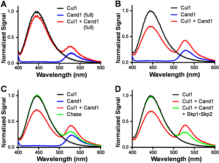
Figure 3: Representative FRET assay for Cul1•Cand1 complex formation. Samples in the FRET buffer (30 mM Tris-HCl, 100 mM NaCl, 0.5 mM DTT, 1 mg/mL ovalbumin, pH 7.6) were excited at 350 nm, and the emissions were scanned from 400 nm to 650 nm. (A) Emission spectra of 70 nM Cul1AMC, 70 nM FlAsHCand1 (full), and a mixture of the two (FRET). Cand1 (full) stands for full length Cand1. (B) Emission spectra of 70 nM Cul1AMC, 70 nM FlAsHCand1, and a mixture of the two (FRET). Cand1 with its first helix deleted was used in this experiment and thereafter. (C) Emission spectra of 70 nM Cul1AMC, 70 nM FlAsHCand1, a mixture of the two (FRET), and chase control for FRET (Chase). The chase sample contained 70 nM Cul1AMC, 700 nM Cand1 and 70 nM FlAsHCand1. (D) Emission spectra of 70 nM Cul1AMC, a mixture of 70 nM Cul1AMC and 70 nM FlAsHCand1 (FRET), and 700 nM Skp1•Skp2 added to the 70 nM Cul1AMC•FlAsHCand1 complex. In each plot, the emission signals were normalized to the emission of 70 nM Cul1AMC at 450 nm. Please click here to view a larger version of this figure.
To measure the kon of Cul1•Cand1 using the established FRET assay by monitoring the reduction of the donor signal over time on the stopped-flow fluorimeter, we first tested and determined the concentration of the protein to be used. When 5 nM each of Cul1AMC and FlAsHCand1 were used, very little signal change was observed (Figure 4A), whereas, when the concentration of each protein was increased to 50 nM, the reduction of the signal over time was observed (Figure 4B) and this change was abolished if buffer without FlAsHCand1 was added (Figure 4C). Therefore, 50 nM Cul1AMC was used for further analyses, and a series of observed association rate constants (kobs) were measured by mixing 50 nM Cul1AMC with increasing concentrations of FlAsHCand1. The kobs for each experiment was calculated by fitting the points to a single exponential curve, and the kobs obtained from the same FlAsHCand1 concentration were averaged. By plotting the average kobs with the Cand1 concentration and performing a linear regression (Figure 4D), the kon was determined7,27.
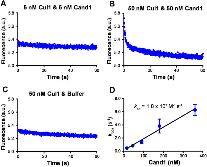
Figure 4: Representative measurement of association rate constant. (A) The fluorescence of 5 nM Cul1AMC was monitored by a stopped-flow fluorimeter over time upon addition of 5 nM FlAsHCand1. (B) The fluorescence of 50 nM Cul1AMC was monitored by a stopped-flow fluorimeter over time upon addition of 50 nM FlAsHCand1. (C) The fluorescence of 50 nM Cul1AMC was monitored by a stopped-flow fluorimeter over time upon addition of the FRET buffer. (D) kon for Cand1 binding to Cul1. kobs of Cul1•Cand1 at different concentrations of Cand1 are plotted. Linear slope gives kon of 1.8 x 10⁷ M-1 s-1. Error bars represent ±SEM; n = 4. All samples were prepared in the FRET buffer and excited at 350 nm. A band-pass filter was used to collect signals from AMC and exclude signals from FlAsH. No data were normalized. Please click here to view a larger version of this figure.
Similar to the measurement of kon, we measured the observed dissociation rate constant of Cul1•Cand1 by monitoring the increase (restore) of the donor signal over time on the stopped-flow fluorimeter. Cul1AMC and FlAsHCand1 were mixed first, and then Skp1•Skp2 was added to the preassembled Cul1AMC•FlAsHCand1 on the stopped-flow fluorimeter. The donor signal increased quickly and it revealed a kobs of 0.4 s-1 (Figure 5). In contrast, when buffer was added to the preassembled Cul1AMC•FlAsHCand1, no signal increase was observed, suggesting the fast dissociation of Cul1•Cand1 was triggered by Skp1•Skp2.
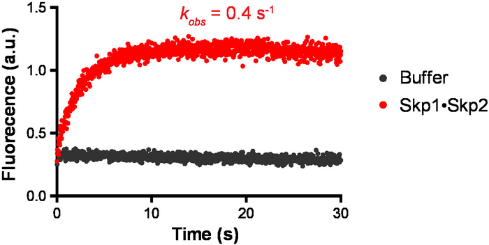
Figure 5: Representative measurement of dissociation rate constant. The change in donor fluorescence versus time was measured following addition of 150 nM Skp1•Skp2 or the FRET buffer to 50 nM Cul1AMC•FlAsHCand1 complex. Signal changes were fit to a single exponential curve, and it gives observed dissociation rate constant of 0.4 s-1. The experimental conditions were similar to that described in Figure 4. Please click here to view a larger version of this figure.