1. Sample preparation
NOTE: Successive steps for preparing the samples are described in Figure 1.
- Plant sample preparation
- From wood trunks or fragments, cut 1 cm long samples with razor blades without damaging their structure.
- Embed samples in polyethylene glycol (PEG) medium, by dipping them in successive solutions of increasing PEG concentration diluted in water until reaching 100% PEG.
- Place sample under vacuum to remove water.
- Gently stir samples in 30% v/v PEG for 24 h.
- Gently stir samples in 50% v/v PEG for 24 h.
- Gently stir samples in 100% PEG for 24 h at 70 °C (pure PEG is solid at room temperature).
- Place samples in capsules at 70 °C (on a hot plate) and progressively decrease temperature until reaching room temperature.
- Prepare carefully 30-60 µm thickness flat sections from these PEG blocks using a microtome and disposables blades.
- Collect and wash sections in three successive baths of water for 5 min to remove PEG from the sections.
- Fluorescent probe preparation
- Prepare buffer solution of 30 mM phosphate at pH 6.0.
- Weigh PEG rhand dextran rhodamine probe powder.
- Dissolve probe powder into the buffer with continuous stirring in a glass vial for 1 h in the dark at a final concentration of 0.1 g/L.
- Plant sample staining
- Incubate sections with 500 µL of the fluorescent probe (see 1.2.3) for 72 h (no stirring) in a plastic tube (no more than 3 sections per tube) in the dark.
- Pick-up a section with a brush, adsorb the buffer with a clean sheet (avoid drying the section), and then mount the incubated sections between a cover glass and a #1.5H coverslip.
2. Fluorescence lifetime and spectral measurement system calibration
NOTE: The complete workflow for sFLIM measurement is presented in Figure 2.
- Determine the spectral window width of the sFLIM detector.
- Put urea crystals in a culture box with a 0.17 µm glass bottom.
- Place the culture box on a microscope sample holder and select the 20x objective.
- Select a Ti:Sa laser with a 900 nm wavelength and 2% power, and turn on the scanning.
- Collect the second harmonic signal on the sFLIM detector.
NOTE: The second harmonic signal is emitted at exactly half excitation wavelength of 450 nm; while instantaneous, this measure also provides the instrumental response function of the system. - Gradually adjust the laser excitation wavelength from 900 to 980 nm until the second harmonic signal is collected in the second spectral channel (462.5 nm).
- Determine the spectral window length (12.5 nm).
- If the spectral range differs from what is expected, troubleshoot by doing the following.
- Adjust the laser to 910 nm.
- Move the grating position with a scroll wheel to measure the second harmonic signal on the first channel only (first channel boundary).
- Adjust the laser to 935 nm.
- Move the grating position with a scroll wheel to measure the second harmonic signal on the first channel only (second channel boundary).
- Calibration of the overall spectrometer channels
- Insert the mirror on the microscope stage.
- Select the visible continuous laser (458 nm, 1% power).
- Collect the reflection signal on the sFLIM detector and check if photons are measured in the appropriate spectral channel.
- Repeat step 2.2.2 and 2.2.3 with all available continuous lasers (514 nm, 561 nm and 633 nm).
- If the spectral channel differs from what is expected, move the grating position with the scroll wheel and repeat steps 2.1 and 2.2.
3. Sample fluorescence characterization
- In a spectrofluorometer equipped with a film holder accessory (e.g., Jasco FP-8500 instrument), place the plant section sample (not incubated with the fluorescent probe).
- Measure fluorescence emission typically on the range 300-600 nm while exciting the sample typically on the range 250-550 nm.
- Plot the fluorescence intensity versus excitation and emission wavelengths to draw a 3D fluorescence map.
- Determine the maximum excitation/emission area from the plot.
4. Spectral FRET measurement
- Autofluorescence calibration
- Select the objective 20x (NA: 0.8).
- Set the two-photon laser excitation at 750 nm.
- Place the wheat straw (WS) alone plant section between the slide and the coverslip.
- Apply the following parameters in the software. Switch to lambda mode. Select the spectral detector ChS with a 9.7 nm resolution. Select the spectral range between 420 to 722 nm.
- Acquire the image.
- Determine the donor emission peak (470 nm with this setup).
- Acceptor's calibration
- Place rhodamine-based fluorescent probes in a culture box with a 0.17 µm glass bottom.
- Acquire the image with the same setting.
- Determine the acceptor emission peak (570 nm with this setup).
- Determine the spectral range with the maximum “WS alone” signal and no acceptor signal as the donor only emission for sFLIM measurements (460-490 nm with this setup).
- Sample measurement
- Place the stained plant section between the slide and the coverslip.
- Acquire the image with the same setting.
- Save the lsm file.
- Qualitatively associate a strong FRET event with a decrease in donor emission peak compared to the “WS alone sample” and an increase in the acceptor emission peak compared to the rhodamine sample.
5. sFLIM measurements
NOTE: For the sFLIM setup, the system used is a time domain sFLIM setup as described previously10. An upright microscope and various time correlated single photon counting cards and confocal microscope manufacturers can be used and the protocol should be adapted accordingly.
- Switch the system to sFLIM mode.
- Set the confocal microscope as described in 4.1.1 and 4.1.2.
- Switch to the Non-Descanned mode in the software to send fluorescent photons to the sFLIM detector.
- Set the sFLIM acquisition to the Enable mode to allow photon counting on the SPC150.
- Select 30 s time collection on SPC150.
- Check that the CFD is between 1 x 10⁵ and 1 x 10⁶.
CAUTION: Ensure that the number of photons measured on the TCSPC card is always less than 1% of the laser excitation frequency (in this setup, the laser excitation frequency is 80 Mhz and detection rate cannot exceed 800 kHz in any pixel to avoid a pile up effect11).
- Place the “WS alone” plant section between the slide and the coverslip.
- Set the software to Continuous mode to allow the laser scan.
- Choose the measurement area on the sample.
- Click Start on the SPC150.
- Save the sdt file.
- Repeat the process for at least 10 samples per condition.
- Place the stained plant section between the slide and the coverslip.
- Repeat steps 5.2.1 – 5.2.5.
6. sFLIM analysis
- Select sFLIM data acquired file on “WS alone” and import them to the SPCImage software using File | Import.
- Select fit parameters.
- From Option | Model, select Incomplete multi-exponentials: 12.5 ns.
- From Option | Preferences, select Calculate Instrumental Response automatically.
- From main panel's right menu, select the 2 exponential fit model:
- For each channel, apply the fitting model and save the fit parameters to a spreadsheet (a1, a2, t1, t2).
- For comparison between channels and experiments, calculate the mean fluorescence lifetime in a spreadsheet (Tm):
- Calculate the mean lifetime for all samples (at least 10) in all channels.
- Analyze Tm on donor channels (from channel 1 to 3: 460-490 nm) and determine the dedicated channel (Channel 2 corresponding to 467.5 – 480 nm) that shows the highest photon number and corresponds to lignin maximum emission. Values from channel 2 must be used in step 6.7.
- Select sFLIM data acquired file on stained WS and import them to the SPCImage software.
- Repeat steps 6.1-6.4.
- Calculate the FRET efficiency EFRET for the donor in the previous selected channel WS Alone (TmD) and from stained plant sample (TmDA):
- Compare sFLIM and EFRET values between the WS and the sample.
- Consider a positive EFRET associated with a homogeneous lifetime decrease between WS and the sample to be analyzed as a FRET event (see representative results and works by Spriet et al.12 and Terryn et al.10 for details).
- Consider a lifetime decrease distributed differently to be due to a mix of FRET and lignin compaction level and do not interpret as molecular interactions.
- Consider no lifetime modification as an absence of measurable FRET signal, but not as a lack of interaction with lignin
To demonstrate the sFLIM capability to dissect molecular interactions between lignin and fluorescently-tagged molecules, we first used three different samples (Figure 3): native wheat straw (WS), native wheat straw incubated with PEG tagged with rhodamine (PR10), and native wheat straw with dextran tagged with rhodamine (DR10). PR10 is known to interact with lignin while DR10 is supposed to be inert13,14,15. sFLIM curves (Figure 3, top) show some modifications that can be achieved between the reference sample (WS) and two interaction cases (DR10 and PR10). Indeed, one can first easily notice the fluorescence increase in spectral regions corresponding to the rhodamine emission range. Careful observation of the three first channel photon decay curves also reveals a stronger inflection for DR10 than for PR10. After fitting the photon decay curves and calculating each channel mean fluorescence lifetime, the FRET signature becomes more obvious (Figure 3, bottom). Indeed, while the fluorescence lifetime alternatively increases and decreases along the fluorescence spectrum for the WS sample, a clear FRET signature is observed for both PR10 and DR10 with: 1) a constant lifetime value in the donor-only emission channel (3 first channels, in blue); and 2) an increasing fluorescence lifetime in the spectral channel corresponding to an increasing contribution of the high lifetime donor fluorophore.
Once unambiguous FRET has been determined, comparison of lignin fluorescence lifetime (channel 2) allows quantification of the lifetime decrease between WS (0.47 ns), DR10 (0.42 ns) and PR10 (0.36 ns) and thus, reveals molecular interactions between lignin and both PR10 and DR10 with a stronger affinity for PR10.
To illustrate the relevance of this method to quantify different interaction levels, we choose three other samples, mimicking enzyme accessibility upon treated plant samples: acid-treated WS (AWS), in combination with PR of two contrasted molecular weights of 5 kDa and 20 kDa (PR5 and PR20). After careful inspection of sFLIM signatures, lignin fluorescence lifetime is extracted (Figure 4). As previously stated, lignin fluorescence lifetime can be altered by its environment16,17. After acid treatment, the fluorescence lifetime measures in AWS (0.28 ns) becomes lower than previously measured for WS (0.47 ns), which confirms the requirement of the sFLIM procedure for unambiguous interpretation of lifetime decrease and the need for negative controls for each tested condition. As expected, a strong lifetime decrease is observed when adding PR to the AWS while it interacts with the lignin. Furthermore, the interaction is stronger with PR5 (0.14 ns) compared to PR20 (0.16 ns), which is consistent with their hydrodynamic radius measurement (2.3 nm and 4.8 nm for PR5 and PR20, respectively), inducing different steric constraints and thus higher accessibility of PR5 to lignin.
Both experiments demonstrate the relevancy of this method to finely assess lignin interactions with enzymes, depending on their size and on plant samples pre-treatment.
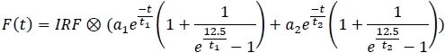
Figure 1: Different preparation steps of the samples. Wheat straw (WS) (A) is first reduced in size (B) to be embedded in PEG medium (C). The block is cut using a microtome equipped with disposable blades (D). After washing, resulting sections (E) are placed for incubation in PEG or dextran tagged-rhodamine solution (F). Labelled sections are mounted for sFLIM measurements (G). Scale bars are 2 cm (A), 1 cm (B and C), 200 µm (E and G). Please click here to view a larger version of this figure.
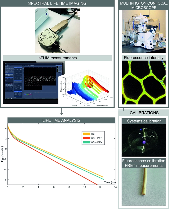
Figure 2: Complete workflow of spectral FRET- based interactions measurements. The figure presents the setup combining spectral fluorescence intensity and lifetime measurements. Spectral fluorescence images are acquired with a confocal microscope, and sequentially fluorescence lifetimes for each spectral range are measured with the sFLIM detector. Analysis of photon decay curves allows accurate determination of interactions between the sample and molecules of interest. Calibrations have to be processed to avoid artefacts. First, the sFLIM detector needs to be spectrally calibrated and its instrumental response function has to be checked. Second, the complex autofluorescence signal has to be precisely calibrated for each sample to determine the fluorescence lifetime in each channel before addition of an acceptor molecule. Please click here to view a larger version of this figure.
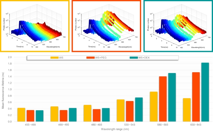
Figure 3: Representative sFLIM measurements. sFLIM curves (top panel) were acquired on native wheat straw (WS), WS incubated with PEG tagged with rhodamine (WS+PEG) and native wheat straw with dextran tagged with rhodamine (WS+DEX). For each sample, sFLIM curves were fitted with a bi-exponential decay model and the mean fluorescence lifetime was calculated for each channel (bottom panel). WS+PEG and WS+DEX samples present a decrease in the fluorescence lifetime in the channel corresponding to autofluorescence only (three first bars) associated with a lifetime increase in channel corresponding to a mixed emission of autofluorescence and rhodamine. This behavior is characteristic of a FRET event between lignin and rhodamine-tagged molecules. Please click here to view a larger version of this figure.
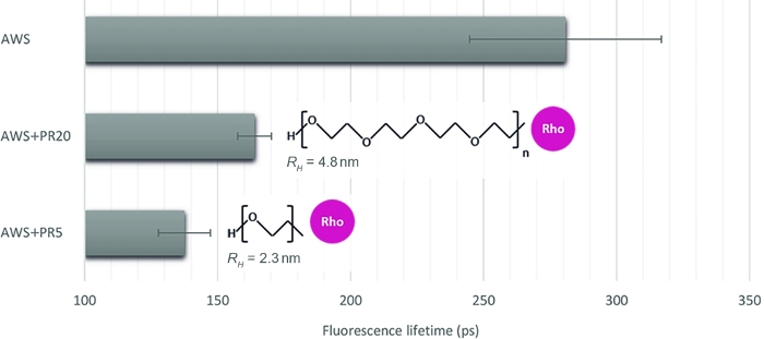
Figure 4: Fluorescence lifetime analysis of the channel corresponding to lignin autofluorescence. After validating a FRET event based on sFLIM signature, mean fluorescence lifetime was measured on acid-treated WS (AWS), in combination with PR5 or PR20 (5 kDa and 20 kDa, respectively). While both PR samples present a lifetime decrease, the smaller is characterized by a stronger lifetime reduction, revealing a stronger molecular interaction with lignin. The method is thus sensitive enough to discriminate between both (mean value and standard error are represented, n>10 per condition). Please click here to view a larger version of this figure.