NOTE: The proteins used in nano-DSF experiments should be pure (>95%) and homogeneous as judged by sodium dodecylsulfate-polyacrylamide gel electrophoresis. Before performing the fragment screen, the stability of the proteins should be determined in various buffer conditions. A low ionic strength, low salt buffer that interferes minimally with the protein should be used so as not to affect its direct interaction with the fragments. The buffers typically used in this protocol for checking stability are shown in Supplemental Table S1. The concentration of the protein that needs to be used for this experiment as a stock solution is typically 0.2 mg mL-1. For screening the entire DSi-Poised library (768 compounds), a total of ~12 mL of protein of that concentration, a total of ~2.5 mg, is needed. The DSi-Poised library used in these experiments was supplied in 96-well format (Figure 1). The concentration of the fragments was adjusted to 100 mM in 20% v/v dimethylsulfoxide (DMSO). It should be noted that the mixing protocol described here results in low final DMSO concentrations of 0.4% v/v; although this is very unlikely to affect the stability of the protein, the effect of DMSO should be checked for each new protein.
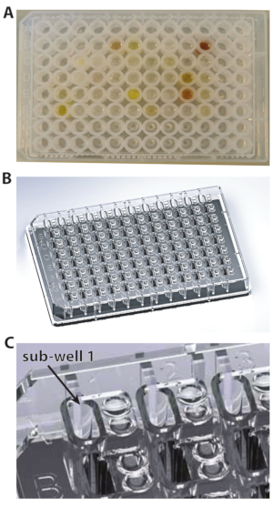
Figure 1: The types of plates used for these experiments. (A) U-bottom plate. (B) 96-well plate. (C) A close-up view of 96-well plate showing the subwell 1. Please click here to view a larger version of this figure.
1. Plate preparation
- Take out a fragment plate from the -20 °C/-80 °C freezer, and let it thaw at room temperature, with gentle shaking on a benchtop shaker. Centrifuge the plate at 500 × g for 30 s to collect any drops sticking to the side of the wells.
NOTE: As the fragment library is available dissolved in DMSO-d6 (melting point 19 °C), it is essential to make sure that each compound is completely thawed and solubilized. - Take an MRC 2-well crystallization plate (Figure 1A), and pipette 14.7 µL of the protein stock solution into each sub-well. To do this in a time-efficient manner, keep the protein in a reagent reservoir (Table of Materials), and use a multichannel pipette for dispensing (Figure 2A,B).
NOTE: For the DSi-Poised library, depending on the format, not all the wells of the 96-well plate contain compounds. Typically, rows A, H and columns 1, 12 are filled with DMSO. Thus, rows A, H and columns 1, 12 are not to be filled with protein, as these wells will not contain any fragments at the end of the next step; only DMSO will be transferred there by the robot. Please note that the empty rows and columns do differ in some plates.
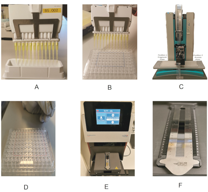
Figure 2: Outline of the fragment screening procedure. (A) Using a multichannel pipette and reagent reservoir to dispense the protein. (B) Dispensing the protein in the 96-well plate. (C) Fragment dispensing by the dispenser robot. (D) Loading of the protein into the capillaries. (E) Drawer showing the capillary holder. (F) Close-up view of the capillary holder. Please click here to view a larger version of this figure.
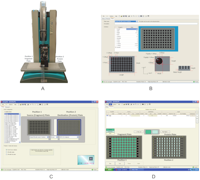
Figure 3: Overview of the equipment used in these experiments. (A) Nanodispenser robot used for fragment dispensing. Plate positions are indicated. (B) Program interface for defining a new plate. (C) Interface of the dispensing program. (D) The dispensing program used to dispense the fragments. Please click here to view a larger version of this figure.
2. Fragment nano-dispensing by the Mosquito robot
- Check the type of plate in which the fragments are supplied (Table of Materials).
- Check fragment and protein plate definitions on the Mosquito.
- Switch on the nanodispenser (Figure 3A). Make sure that there are no obstacles around the moving components.
- Open the graphical user interface, click on the Setup tab, and under Deck Configuration, check whether the type of plate in which the compounds are supplied and the one in which the protein has been transferred in section 1 are already present in the list of the Available plates. If not, click Options|Plates and create a new plate definition by filling in the correct values for the Property type (Figure 3B).
NOTE: These values for the MRC 2-well plate and the 96-well plate used in this experiment are shown in Supplemental Table S2 and Supplemental Table S3, respectively.
- The dispensing program
- Under the Setup tab, specify the plate positions under Deck Configuration.
NOTE: The Mosquito used in this experiment has two plate positions on the deck. Position 1 is defined as the Source plate, and Position 2 is the Destination plate. - Using the dropdown menu, choose Greiner U bottom plate for Position 1 and MRC 2-well plate for Position 2 (Figure 2C). Save the protocol.
- Under the Setup tab, specify the plate positions under Deck Configuration.
- Fragment dispensing
- Place the fragment plate at Position 1 and the protein plate at Position 2 of the deck (Figure 3A).
- On the Protocol tab (Figure 3D), click on File and choose the protocol saved in section 2.3 for dispensing the fragments. Define the volume of the fragments to be dispensed; use 0.3 µL. For a typical plate, where columns 1 and 12 do not contain fragments, define the Start location to column 2 and the End location to column 11. In some plates, if columns 2 or 11 are empty, use columns 3 and 10 as start and end values, respectively.
NOTE: Because of the Mosquito setup, only columns can be skipped, not rows; for the rows, the mosquito will pipette DMSO. Make sure that the Tip Changing option is selected as Always, so as not to cross-contaminate the fragment library. - Click on Run to start the program. After dispensing, which takes ~2 min, is completed, remove the protein and the fragment plates from the robot, and seal them back with an adhesive sealing film. Briefly centrifuge the protein plate (500 × g, 30 s) to collect any drops sticking to the sides of the wells before proceeding to the next step.
3. Measurement of nano-DSF
NOTE: A detailed description about performing TSAs using the Prometheus NT.48 has been published previously20. Important points in the context of fragment screening are mentioned here.
- Plate inspection before the measurement
- Visually inspect the wells of the protein plate for precipitation that might have occurred due to the addition of the fragments. If precipitation is observed in many wells, reduce the concentration of the fragments, and repeat the experiment.
NOTE: It is recommended to keep the protein plate at room temperature; the fragments tend to become insoluble at lower temperatures.
- Visually inspect the wells of the protein plate for precipitation that might have occurred due to the addition of the fragments. If precipitation is observed in many wells, reduce the concentration of the fragments, and repeat the experiment.
- Preparing the Prometheus
- Switch on the Prometheus instrument. On the touchscreen, press Open Drawer to access the capillary loading module of the instrument. Remove the magnetic strip from the loading module, and clean the mirror with ethanol to remove any dust particles.
- Transfer from the protein-fragments plate to capillaries
NOTE: This step involves transferring the mixed protein/fragment sample from each well in the protein plate to the capillaries for use with the Prometheus. For this, although the Standard capillary type is typically used, it is possible to use the High Sensitivity capillaries for very low protein concentrations.- Place the protein plate and the capillaries next to the instrument to have easy access to the capillary loading module.
- Take one capillary, hold it at one end, and touch the solution in the protein plate with the far end of the capillary to transfer the sample by capillary action. Always wear gloves, and make sure not to touch the capillary in the middle, as impurities (e.g., dust particles) from the gloves would affect the measurement.
- Place the capillary in the designated position of the holder, making sure it is properly aligned and centered.
- Repeat steps 3.3.2 and 3.3.3, thereby filling up all positions in the loading module. Load all capillaries you will need for measurement.
NOTE: For a single run, a maximum of 48 capillaries can be loaded. - At the end, place the magnetic strip on top of the capillaries to hold them in place, and press Close Drawer to start the experiment.
- Perform the nano-DSF experiment
- Fluorescence scan
- Open the Prometheus application PR.ThermControl, and create a new project by clicking on Start New Session using the name ProteinName_ScreenName_PlateNumber. First, do a Discovery Scan to detect the fluorescence of the samples.
NOTE: The fluorescence levels should ideally be above 3,000 counts for each sample. Samples having fluorescence above the saturation limit of the instrument (20,000 counts) will not be measured. - Alter the fluorescence signal of the samples by adjusting the Excitation Power of the laser (Figure 4).
- Open the Prometheus application PR.ThermControl, and create a new project by clicking on Start New Session using the name ProteinName_ScreenName_PlateNumber. First, do a Discovery Scan to detect the fluorescence of the samples.
- Thermal denaturation
- Click on the Melting Scan tab. To perform the experiment, set the Start Temperature to 20 °C, the End Temperature to 95 °C, and the Temperature Slope to 1 °C min-1. Click on Start Measurement.
- Annotating the experiment
- After the experiments starts, click on the Annotation and Results tab. Annotate each capillary by giving it a unique plate- and well-number.
NOTE: For example, capillary 1B2 would correspond to Plate 1 and well B2. In this tab, extra columns can be added for the experiment, e.g., protein name, buffer, protein concentration. After the experiment is finished, the results are also displayed in this tab. This is a good time to pause at the end of the day; the experiments take place overnight, the results can be collected the next day.
- After the experiments starts, click on the Annotation and Results tab. Annotate each capillary by giving it a unique plate- and well-number.
- Data visualization and export
- After the experiment is finished, click on the Melting Scan tab to view the melting and scattering curves for the samples. To export the results in a spreadsheet, click on the Melting Scan tab, click on Export, and choose Export Processed Data from the drop-down menu.
- Fluorescence scan
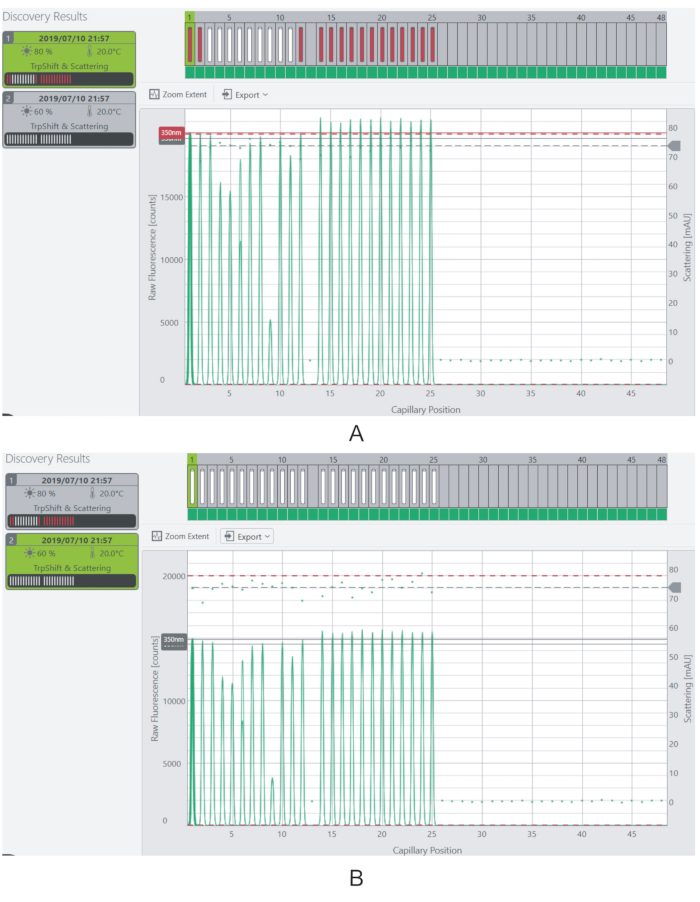
Figure 4: Adjusting the excitation power and fluorescence signal. (A) At 80% excitation power, the fluorescence signal for most of the samples is beyond the saturation limit. (B) The fluorescence signal is reduced to measurable levels by decreasing the excitation power to 60%. Please click here to view a larger version of this figure.
4. Iteration
- Repeat steps 1-3 to perform 16 runs on the entire Enamine library of 768 compounds (16 × 48 = 768).
- As the measurement of each plate takes ~1.5 h to complete, complete the annotation (3.4.3), and prepare the next protein-fragments plate by repeating steps in sections 1 and 2.
NOTE: In a typical working day, 4-6 plates can be measured, depending on experience. The screening of the entire DSi-library can be finished in a total of 3-4 days.
5. Data analysis
- Examining the generated data
- Once each run is completed, click on the Annotations and Results tab to display the results. For each sample, focus on two calculated values that are most important in this overview: 1) The scattering onset temperature (Onset #1 for Scattering), which indicates the temperature at the start of increased sample scattering events and is characteristic of aggregation; 2) the Tm (Inflection Point #1 for Ratio) value extracted from the ratio between fluorescence events at 330 and 350 nm-values that typically correspond to the maximal changes of tryptophan fluorescence upon changes in its environment.
- Be sure to check the scattering and the melting curves for each capillary in the Melting Scan tab to make sure that these values are reliable.
- Export and inspection to a spreadsheet
- Export the data from all different runs for inspection to a spreadsheet software, as described in 3.4.4, and to create overview tables and plots. Click on the various Sheets in the spreadsheet file to note the information in each sheet.
- In the Overview sheet, note that each row corresponds to one experiment. Along an overview of parameters (e.g., start and end temperature), observe the calculated values for the Tm and the scattering onset (see 5.1 above for names and explanation, and Supplemental files 1 and 2 for an example). As the software calculates two or more Tm values (Inflection Point #1 and #2 for Ratio) for some samples, look at the melting transition curve to determine which of the Tm values is correct.
- In the Ratio sheet, note that each column corresponds to a sample, and each row to the data read at each temperature step. Observe the fluorescence count values corresponding to each temperature step, and use them to plot the melting curves for specific samples, plotting the temperature column against the fluorescence count column. Note that the data in the Ratio (first derivative), 330 nm, 330 nm (first derivative), 350 nm, 350 nm (first derivative) are used to calculate the ratio and its first derivative (which has a maximum at the maximum rate of change) in a similar format.
- Observe similar data for scattering in the Scattering sheet. Generate the scattering curve for each sample by plotting the temperature column against the scattering column. Look for the Sheet for the scattering first derivative.
- Export the data from all different runs for inspection to a spreadsheet software, as described in 3.4.4, and to create overview tables and plots. Click on the various Sheets in the spreadsheet file to note the information in each sheet.
- Creating and validating a global overview for all fragments
- After verifying the correct Tm values for the fragments, combine the columns Sample ID and Inflection point of 330/350 nm ratio (Tm) from all the runs in a single new result file, copying these columns from each run.
- Use the average Tm value of the native protein (typically calculated over ten runs) and subtract it from the Tm values of each sample, to get the ΔTm. Sort the results over ΔTm in descending order to identify the samples that result in the largest shift.
- Divide the fragments into bins depending on the ΔTm shift, and generate a frequency table for the whole library by plotting the ΔTm for each bin against the number of fragments (Figure 5). For convenience, show the axis representing the number of fragments in the log scale. Bin the sample with ΔTm ±1, and adapt the other bins to each run to adjust the number of outliers empirically.
A full screen of the DSi-Poised library (768 fragments) was performed on three proteins of medical interest, namely, the outer kinetochore Highly Expressed in Cancer 1 protein (Hec1, or Ndc80), the regulatory tetraricopeptide repeat (TPR) domain of the monopolar spindle kinase 1 (Mps1), and the SARS-CoV-2 3C-like protease, Nsp5, which cleaves off the C-terminus of the replicase polyprotein at 11 sites. The buffer conditions chosen for each protein, as well as the protein concentration and Tm of the proteins, are shown in Supplemental Table S4.
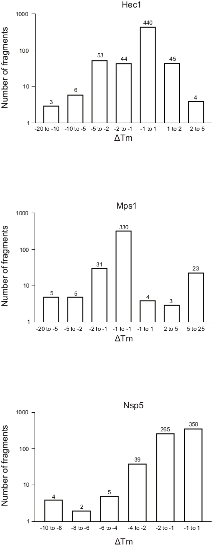
Figure 5: Frequency distribution of the shift in melting temperature (ΔTm) for the three proteins, Hec1, Mps1, and Nsp5, presented in this study as representative results. Abbreviations: Hec1 = Highly Expressed in Cancer 1 protein; Mps1 = monopolar spindle kinase 1; Nsp5 = SARS-CoV-2 3C-like protease. Please click here to view a larger version of this figure.
The results of the three screenings using the protocol described above, displayed as the frequency distribution of the change in Tm versus the number of fragments, are shown in Figure 5. These plots have been generated as described in section 5.3 of the protocol, plotting the frequency of the observed change in Tm. The significance of the shift needs to be defined in a subjective manner for every different project, as described in the discussion section below. Negative values indicate a reduction in the melting temperature in the presence of a fragment, a positive value an increase in Tm. From such plots, it is easy to observe that for Nsp5, all the fragments have a destabilizing effect, whereas for Hec1 and Mps1, both stabilizing and destabilizing hits are observed. This can be expected and will be discussed.