1. Experimental Protocol
- Sample preparation
NOTE: Perform cell seeding and transfection under sterile conditions.- Place a cleaned coverslip per well into a 6-well culture plate and wash three times with sterile phosphate-buffered saline (PBS).
NOTE: The coverslip cleaning protocol is detailed in Supplementary Note 1. - To each well, add 2 mL of the complete cell culture medium containing phenol red (supplemented with 10% fetal bovine serum (FBS), 100 µg/mL penicillin and 100 µg/mL streptomycin) and keep the plate aside.
- Culture the CHO cells in the same medium containing phenol red at 37 °C and 5% CO2. Wash the cells with 5 mL of PBS to remove the dead cells.
- Add 2 mL of trypsin and incubate for 2 min at room temperature (RT).
- Dilute the detached cells with 8 mL of medium containing phenol red and mix carefully by pipetting.
- Count the cells in a Neubauer chamber and seed at a density of 1.5 x 10⁵ cells/well in the 6-well cell culture plate containing the coverslips (prepared in step 1.1.1-1.1.2).
- Let the cells grow in an incubator (37 °C, 5% CO2) for 24 h in order to achieve approximately 80% confluency.
- Dilute 2 µg of the desired vector DNA (e.g., CT-SNAP or NT-SNAP) and 6 µL of the transfection reagent in two separate tubes, each containing 500 µL of the reduced-serum medium for each well and incubate for 5 min at RT.
- Mix the two solutions together to obtain the transfection mixture and incubate it for 20 min at RT.
- In the meantime, wash the seeded CHO cells once with sterile PBS.
- Replace the PBS with 1 mL/well of phenol red-free medium supplemented with 10% FBS without any antibiotics.
- Add the entire 1 mL of transfection mixture dropwise to each well and incubate the cells overnight at 37 °C, in 5% CO2.
- For labeling of the SNAP construct, dilute the appropriate SNAP substrate stock solution in 1 mL of the medium supplemented with 10% FBS to obtain a final concentration of 1 µM.
- Wash the transfected cells once with PBS and add 1 mL per well of 1 µM SNAP substrate solution. Incubate the cells for 20 min at 37 °C in 5% CO2.
- Wash the cells thrice with phenol red-free medium and add 2 mL per well phenol red-free medium. Incubate the cells for 30 min at 37 °C in 5% CO2.
- Transfer the coverslips of all samples subsequently into the imaging chamber and wash with 500 µL imaging buffer. Add 500 µL imaging buffer before moving to the FRET-FCS setup.
- Place a cleaned coverslip per well into a 6-well culture plate and wash three times with sterile phosphate-buffered saline (PBS).
- Calibration Measurements
NOTE: The FRET-FCS setup is equipped with a confocal microscope water objective, two laser lines, a Time-Correlated Single Photon Counting (TCSPC) system, two hybrid photomultiplier tubes (PMT) and two avalanche photodiodes (APD) for photon collection and the data collection software. It is very important to align the setup every time before live cell measurements. The detailed setup description can be found in Supplementary Note 2. Both lasers and all detectors (two PMTs and two APDs) are always ON during the measurements, as all measurements need to be conducted under identical conditions. For the calibration measurements, use a coverslip from the same lot on which the cells were seeded, this decreases the variation in collar ring correction.- For adjusting the focus, pinhole and collar ring position, place 2 nM green calibration solution on a glass coverslip and switch on the 485 nm and 560 nm laser. Operate laser in Pulsed Interleaved Excitation (PIE) mode16.
- Focus on the solution and adjust the pinhole and collar ring position such that the highest count rate and smallest confocal volume are obtained to get the maximum molecular brightness.
- Repeat this process for the red channels with 10 nM red calibration solution and a mixture of both, the green and red calibration solution.
- Place the 10 nM DNA solution on a glass coverslip and adjust the focus, pinhole, and collar ring position such that the cross-correlation between the green and red detection channels is highest, i.e., shows the highest amplitude.
NOTE: Steps 1.2.1 and 1.2.4 might have to be repeated back and forth to find the optimal alignment. Take 3-5 measurements from each calibration solution for 30 s – 120 s after the focus, pinhole, and collar ring position have been aligned optimally for the green and red detection channels and the confocal overlap volume. - Measure a drop of ddH2O, the imaging medium, and a non-transfected cell 3-5 times each for 30 s – 120 s to determine the background count rates.
- Collect the instrument response function with 3-5 measurements for 30 s – 120 s. This is optional but highly recommended.
- Live cell measurements
- Find a suitable cell by illuminating with the mercury lamp and observing through the ocular.
NOTE: Suitable cells are alive showing the typical morphology of the respective adherent cell line. The fluorescence of the protein of interest, here a surface receptor, is visible all over the surface. Less bright cells are more suitable than brighter ones due to the better contrast in FCS when a low number of molecules are in focus. - Switch on both lasers in PIE mode and focus on the membrane by looking at the maximum counts per second.
NOTE: The laser power might need to be reduced for the cell samples (less than 5 µW at objective). This depends upon the used fluorophores and the setup. - Observe the auto- and cross-correlation curves of the eGFP or labelled SNAP-tag attached to the β2AR in the online preview of the data collection software and collect several short measurements (~2 -10) with an acquisition time between 60 -180 s.
NOTE: Do not excite the cells for a long time continuously as the fluorophores may bleach. However, it will depend on the brightness of each cell, how long the measurements can be, and how many measurements in total can be performed.
- Find a suitable cell by illuminating with the mercury lamp and observing through the ocular.
2. Data analysis
- Data Export
- Export the correlation curves, G(tc), and count rates, CR, from all measurements.
- Take care to correctly define the "prompt" and "delay" time windows and use the "microtime gating" option in the data correlation software.
NOTE: In total, three different correlations are required: (1) autocorrelation of the green channel in the prompt time window (ACFgp), (2) autocorrelation of the red channels in the delay time window (ACFrd), and finally (3) the cross-correlation of the green channel signal in the prompt time window with the red channel signal in the delay time window (CCFPIE). The data export is shown step-by-step for different software in Supplementary Note 3.
- Calibration measurements
- Use the autocorrelation functions of the green (ACFgp) and red (ACFrd) fluorophore solutions, and fit them to a 3D diffusion model with an additional triplet term if required (eq. 1) to calibrate the shape and size of the confocal detection volume for the two used color channels:
 eq. 1
eq. 1
Here, b is the baseline of the curve, N the number of molecules in focus, tD the diffusion time (in ms), and s = z0/w0 the shape factor of the confocal volume element. The triplet blinking or other photophysics is described by its amplitude aR and relaxation time tR.
NOTE: All variables and symbols used within the protocol are listed in Table 1. - Use the known diffusion coefficients D for the green26 and red calibration standard27 and the obtained shape factors sgreen and sred to determine the dimensions (width w0 and height z0) and volume Veff of the confocal volume element (eq. 2a-c).
 eq. 2a
 eq. 2b
 eq. 2c
NOTE: Templates for calculation of the calibration parameter are provided as supplementary files (S7). - Calculate the spectral crosstalk α of the green fluorescence signal (collected in channels 0 and 2) into the red detection channels (channel number 1 and 3) as a ratio of the background-corrected (BG) signals (eq. 3).
eq. 3 - Determine the direct excitation of the acceptor fluorophore δ by the donor excitation wavelength by the ratio of the background-corrected count rate of the red calibration measurements in the "prompt" time window (excitation by green laser) to the background-corrected count rate in the "delay" time window (excitation by red laser) (eq. 4).
eq. 4 - Calculate the molecular brightness B of both the green and red fluorophores (eq. 5a-b) based on the background-corrected count rates and the obtained number of molecules in focus, N, from the 3D diffusion fit (eq. 1):
 eq. 5a
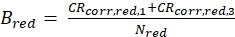 eq. 5b
 - Fit both ACFgp and ACFrd as well as CCFPIE of the double-labeled DNA to the 3D diffusion model (eq. 1). Keep the obtained shape factors, sgreen and sred, constant for ACFgp and ACFrd, respectively. The shape factor for the CCFPIE, sPIE, is usually in between these two values.
NOTE: In an ideal setup, both Veff,green and Veff, red would have the same size and overlap perfectly. - Determine the amplitude at zero correlation time, G0(tc), based on the found values of the apparent number of molecules in focus (Ngreen, Nred and NPIE).
- Calculate the amplitude ratio rGR and rRG for a sample with 100% co-diffusion of green and red fluorophores (eq. 6). Be aware that NPIE does not reflect the number of double-labeled molecules in focus but reflects only the 1/G0(tc).
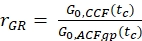 and
and 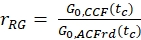 eq. 6
eq. 6
- Use the autocorrelation functions of the green (ACFgp) and red (ACFrd) fluorophore solutions, and fit them to a 3D diffusion model with an additional triplet term if required (eq. 1) to calibrate the shape and size of the confocal detection volume for the two used color channels:
- Live cell experiments
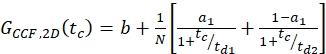
- For single-labeled constructs, fit the cell samples to an appropriate model. For the shown membrane receptor, diffusion occurs in a bimodal fashion with a short and a long diffusion time. Additionally, the photophysics and blinking of the fluorophores have to be considered:
 eq. 7
eq. 7
Here, td1 and td2 are the two required diffusion times, and a1 is the fraction of the first diffusion time.
NOTE: In contrast to the calibration measurements, in which the free dyes and DNA strands freely diffuse in all directions, the membrane receptor shows only 2D diffusion along the cell membranes. This difference between 3D and 2D diffusion is reflected by the modified diffusion term (compare eq. 1), where tD in the 2D case does not depend upon the shape factor s of the confocal volume element. - Calculate the concentration c of green or red labeled proteins from the respective N and Veff using basic math (eq. 8):
 eq. 8
eq. 8
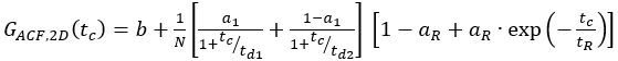
where NA = Avogadro's number - For N-terminal SNAP label and intracellular eGFP, fit the two autocorrelations (ACFgp and ACFrd) of the double-labeled sample using the same model as for the single-labeled constructs for the ACFs (eq. 7) and the CCFPIE using a bimodal diffusion model (eq. 9):
 eq. 9
eq. 9
NOTE: For a global description of the system, all three curves have to be fit jointly: The diffusion term is identical for all three curves and the only difference is the relaxation term for the CCFPIE. As photophysics of two fluorophores is usually unrelated, no correlation term is required. This absence of relaxation terms results in a flat CCFPIE at short correlation times. However, crosstalk and direct excitation of the acceptor due to the donor fluorophore might show false-positive amplitudes and should be carefully checked for using the calibration measurements. - Calculate the concentration c of green or red labeled proteins from the respective N and Veff using equation 8.
- Estimate the fraction or concentration, cGR or cRG, of interacting green and red labeled proteins from the cell samples using the correction factors obtained from the DNA samples, the amplitude ratios rGR and rRG of the cell sample and their respective obtained concentrations (eq. 10).
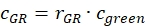 and
and 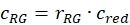 eq. 10
 - For C-terminal SNAP label and intracellular eGFP, fit the two autocorrelations (ACFgp and ACFrd) of the FRET sample as the single-labeled samples (equation 7) and the CCFFRET to a bimodal diffusion model containing an anti-correlation term (equation 11)
 eq. 11
where af reflects the amplitude of the total anti-correlation and aR and tR the respective amplitude and relaxation time.
NOTE: In case of anti-correlated fluorescence changes due to FRET, one or several anti-correlation terms might be required (eq. 11), resulting in a "dip" of CCFFRET at low correlation times coinciding with a rise in the two autocorrelations (ACFgp and ACFrd). However, be aware that photophysics such as triplet blinking might mask the anti-correlation term by dampening the FRET-induced anti-correlation. A joint analysis supplemented with filtered FCS methods might help to unmask the anti-correlation term. Additionally, technical artifacts stemming from dead times in the counting electronics in the nanoseconds range should be excluded16. A more detailed step-by-step procedure on how to perform the analysis in ChiSurf28 and templates for the calculation of confocal volume or molecular brightness are provided on the Github repository (https://github.com/HeinzeLab/JOVE-FCS) and as supplementary files (Supplementary Note 4 and Supplementary Note 6). Additionally, the python-scripts for batch export of data acquired with the Symphotime software in .ptu format can be found there.
- For single-labeled constructs, fit the cell samples to an appropriate model. For the shown membrane receptor, diffusion occurs in a bimodal fashion with a short and a long diffusion time. Additionally, the photophysics and blinking of the fluorophores have to be considered:
Exemplary results of the calibration and live-cell measurements are discussed below. Additionally, the effect of FRET on the cross-correlation curves is demonstrated based on simulated data next to the effect of protein-protein-interaction increasing the CCFPIE amplitude.
PIE-based FCS data export
In PIE experiments, data are collected in the time-tag time-resolved mode (TTTR)29,30. Figure 1B shows the photon arrival time histograms of a PIE measurement of a double-labeled DNA strand on the described setup (Supplementary Note 1). The setup has four detection channels. The fluorescence emission is first split by polarization in "S" and "P" directions (referring to the perpendicular and parallel plane in which the electric field of a light wave is oscillating). Secondly, each polarization direction is then split in two color channels (green, red) before detection, resulting in four channels (S-green, S-red, P-green, P-red). In the "prompt" time window, the green fluorophore gets excited, and the signal is detected in both the green and red channels due to FRET. In the delay time window, only the red fluorophore (in the red channel) is visible. Based on the detection channels and "prompt" versus "delayed" time windows, at least five different correlation curves (3 autocorrelation curves (ACFs) and 2 cross-correlation curves (CCFs)) can be obtained (Figure 1C-D): (1) green signal in the prompt time window (ACFgp), (2) red signal in the prompt time window (in case of FRET, ACFrp), and (3) red signal in the delay time window (ACFrd). These ACFs report on the protein mobility, photophysics (e.g., triplet blinking) and other time-correlated brightness changes in the fluorophores (e.g., due to FRET). (4) The PIE-based cross-correlation CCFPIE of the green signal in the prompt time window with the red signal in the delay time window allows determining the fraction of co-diffusion of the green and red fluorophore16. (5) The FRET-based cross-correlation CCFFRET of the green with the red signal in the prompt time window is related to FRET-induced, anticorrelated brightness changes in the green and red signals31,32,33.
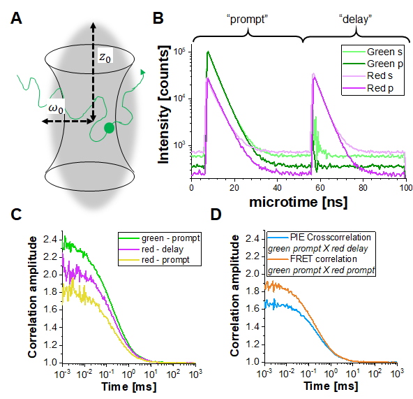
Figure 1: Pulsed-interleaved excitation (PIE) based fluorescence (cross) correlation spectroscopy (F(C)CS). (A) In FCS fluorescently labeled molecules diffuse freely in and out of a (diffraction-limited) focal volume shaped by a focused laser beam that induces fluorescence within this tiny volume. The resulting intensity fluctuations of molecules entering and leaving the volume are correlated and provide information on the mobility of the molecules. (B) In PIE, two different laser lines ("prompt" and "delay") are used to excite the sample labeled with two different fluorophores ("green" and "red"). The time difference between both excitation pulses is adapted to the fluorescence lifetimes of the respective fluorophores so that one has decayed before the other is excited. In the double-labeled sample shown, both fluorophores are sufficiently close to undergo Förster Resonance Energy Transfer (FRET) from the "green" donor fluorophore to the "red" acceptor fluorophore. Thus, red fluorescence emission can be detected in the "prompt" time-window upon excitation of the green donor. In the used setup (Supplementary Note 2), two detectors are used for each color, one oriented parallel to the excitation beam orientation (denoted "p") and the second perpendicular (denoted "s"). (C) Three different autocorrelation functions can be determined in a PIE experiment: Correlation of the i) green channel signals in the prompt time window (ACFgp), ii) red channel signals in the prompt time window (ACFrp) and iii) red channel signals in the delay time window (ACFrd). (D) Two different cross-correlation functions can be determined: iv) The "PIE" cross-correlation (CCFPIE) with green channel signals in the prompt time window correlated with the red channel signals in the delay window, where the amplitude of this curve is related to the co-diffusion of fluorophores; and v) the "FRET" cross-correlation (CCFFRET) with the green channel signals in the prompt time window correlated with the red channel signals in the same prompt window; here the shape of this curve at times faster than diffusion is related to the FRET-induced intensity changes. Please click here to view a larger version of this figure.
Calibration
Figure 2A-B shows a calibration measurement of the singly diffusing green and red fluorophores, respectively. Based on a fit with eq. 1 and the known diffusion coefficient Dgreen26 and Dred27 the shape (z0 and w0) and size (Veff) of the detection volume are calculated using eq. 2a-c. The fit results from the ACFgp from the green fluorophore and ACFrd from the red fluorophore are summarized in Figure 2C. Both fluorophores show an additional relaxation time constant of 8.6 µs (18%) and 36 µs (15%), respectively. The molecular brightness (eq. 5a-b) of the green and red fluorophore amounts to 12.5 kHz per molecule and 2.7 kHz per molecule, respectively.
For a reliable estimation of the confocal volume size and shape as well as the molecular brightness, it is recommended to perform 3-5 measurements per calibration experiments and a joint (or global) fit of all repeats.
The crosstalk α (Figure 2D, eq. 3) and the direct excitation of acceptor by the green laser δ (Figure 2E, eq. 4) for this fluorophore pair lie at ~15% and ~ 38%, respectively.
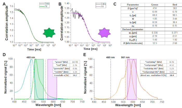
Figure 2: Calibration measurements of freely diffusing green and red calibration standard. (A-B) Representative 60 s measurement of a 2 nM green (A) and a 10 nM red (B) calibration standard measurement fitted to the 3D diffusion model including an additional relaxation time (eq. 1). The table in panel (C) shows the fit results and the derived parameter based on eq. 2a-c and eq. 5a-b. *Diffusion coefficients were taken from literature26,27. (D) Determination of the crosstalk α of the green signal into the red channels (eq. 3). The excitation spectrum of the green standard is shown in cyan, the emission spectrum in green. The excitation laser lines at 485 nm (blue) and 561 nm (orange) are shown as dashed lines. Transparent green and magenta boxes show the collected emission range (Supplementary Note 2). (E) Determination of the direct excitation δ of the red fluorophore by the 485 nm laser (eq. 4). Color code is identical to (D), light and dark orange show the excitation and emission spectrum of the red standard, respectively. Please click here to view a larger version of this figure.
To determine and calibrate the overlap of the green and red excitation volume, a double-labeled DNA double strand is used (Figure 3A) as described above. Here, the fluorophores are spaced 40 bp apart such that no FRET can occur between the green and red fluorophores attached to the ends of the DNA double strands. Figure 3B shows the autocorrelations from both fluorophores in green (ACFgp) and magenta (ACFrd) and the PIE-cross correlation, CCFPIE, in cyan. Please note that for CCFPIE, the signal in the green channels in the prompt time window is correlated with the signal in the red channels in the delay time window16.
Here, an average diffusion coefficient for the DNA strand of DDNA = 77 µm²/s is obtained. More details on the calculation can be found in the step-by-step protocol, Supplementary Note 4. This value is obtained by inserting the calibrated green and red detection volumes size (Figure 2) and the respective diffusion times of ACFgp and ACFrd of the DNA strand (Figure 3C) into equation 2a. Next, using the obtained correction values rGR and rRG and using eq. 6 later on, the amount of co-diffusion, i.e., double-labeled molecules (or protein complexes in case of co-transfection of two different proteins) can be determined from the cell samples.
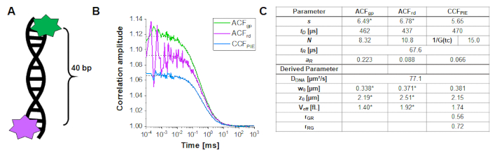
Figure 3: Calibration of the green-red overlap volume using a DNA sample. (A) The DNA strand used for calibration carries a green and a red calibration fluorophore, with a distance of 40 bp in between. The interdye distance must be sufficiently large to exclude FRET between the fluorophores. (B) Representative 60 s measurement of a 10 nM DNA solution. Autocorrelations from both fluorophores in green (ACFgp, green standard) and magenta (ACFrd, red standard) and the PIE-crosscorrelation, CCFPIE, in blue. The table in panel (C) shows the fit results based on the 3D Diffusion model including an additional relaxation term (eq. 1) and the derived parameter diffusion coefficient of DNA, DDNA (eq. 2a), the size and shape of the overlap volume (eq. 2a-c) and the correction ratios rGR and rRG (eq. 6). Please note the values for the green and red detection volume (labeled with *) were taken from the fit of the individual fluorophores shown in Figure 2. Please click here to view a larger version of this figure.
Live-cell experiments
In the following section, the analysis of live-cell experiments for different β2AR constructs is presented. As β2AR is a membrane protein, its diffusion is largely limited to a two-dimensional diffusion (Figure 4A) along the cell membrane (except for transport or recycling processes to or from the membrane) 2. With the restriction to the 2D diffusion the shape factor s = z0/w0 in eq. 1 becomes obsolete resulting in a simplified diffusion model (eq. 9).
Single-labeled constructs: β2AR-IL3-eGFP and NT-SNAP-β2AR
Figure 4 shows exemplary measurements of the single-label construct β2AR-IL3-eGFP (Figure 4B), where eGFP is inserted into the intracellular loop 3, and the construct NT-SNAP-β2AR (Figure 4C), where the SNAP tag is conjugated to the N-terminus of β2AR. The SNAP tag is labeled with a membrane-impermeable SNAP surface substrate. The representative curves show the average of 4-6 repeated measurements with acquisition times of 120 – 200 s each. The respective autocorrelations ACFgp and ACFrd of the eGFP and SNAP signal are fitted to a bimodal, two-dimensional diffusion model (eq. 9). In terms of fast dynamics, eGFP shows only the expected triplet blinking at tR1 ~ 9 µs while the SNAP signal requires two relaxation times, one at the typical triplet blinking time of tR1 ~ 5 µs and a second one at tR2 ~ 180 µs.
The molecular brightness of the fluorophores in living cells is 0.8 KHz (eGFP) and 1.7 kHz (SNAP) per molecule under the given excitation conditions (eqs. 5a-b). The concentration of the labeled β2AR constructs incorporated in the cell membrane should be in the nano-molar range and can be determined by the average number of molecules (eq. 9, Figure 4C) and the size of the respective confocal volume for the green and red channel (Figure 2) using eq. 8.
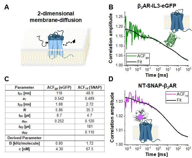
Figure 4: Representative measurement of single-label constructs. (A) In this study, the membrane receptor β2AR was used as an example. In contrast to the fluorophores and DNA strand used for calibration, which could freely float through the detection volume, membrane proteins diffuse mainly laterally along the membrane, described as 2-dimensional diffusion. (B, D) ACFgp and ACFrd of the single-label constructs β2AR-IL3-eGFP (B) and NT-SNAP-β2AR (D). Shown is the average of 4-6 measurements each collected for 120 – 200 s. The table in panel (C) shows the fit results of the data to the bimodal two-dimensional diffusion model including additional relaxation terms (eq. 7). Please click here to view a larger version of this figure.
Double-labeled construct: NT-SNAP-β2AR-IL3-eGFP
In the double-labeled construct NT-SNAP-β2AR-IL3-eGFP (short NT-SNAP), eGFP is inserted into the intracellular loop 3, and, the SNAP tag conjugated to the N-terminus of β2AR (Figure 5A). In this configuration, the eGFP is on the inner side of the membrane and the SNAP on the outer side with too large distances for FRET. In an ideal case, this construct would show 100% co-diffusion of the green and red fluorophore, and no FRET signal. Figure 5B-D shows two measurements of the NT-SNAP in two cells on two different measurement days. Fitting the ACFgp and ACFrd of the "better" measurement shown in Figure 5B with eq. 7 and the CCFPIE with eq. 9, reveals 50- 60 molecules in focus for the ACFgp and ACFrd, whereas Napp, thus 1/G0(tc) ~ 114 for the CCFPIE (Figure 5C). The concentration of labeled receptors lies in the ~100 nM range as determined with eq. 8. To determine the average concentration of double-labeled molecules, first, the ratio of G0(tc) (represented by 1/N(app)) of the CCFPIE to ACFgp and ACFrd, respectively, is calculated (eq. 6). Next, these values, rGRcell= 0.43 and rRGcell = 0.53 are compared to the values obtained from the DNA measurement (rGR,DNA= 0.51 and rRG,DNA = 0.79 on this measurement day). Using the rule of proportions, a rGRcell= 0.43 from the ACFgp of the eGFP signal reflects to a fraction of co-diffusion (rGRcell/rGR,DNA) of 0.84, where for the other case of ACFrd of the SNAP substrate signal, this value amounts to 0.67. The average concentration of the double-labeled NT-SNAP construct can finally be calculated based on eq. 10. In contrast, in the measurement shown in Figure 5D from a different day, the concentration of receptors is quite low and the data very noisy such that the fit range is limited up to ~ 10 µs. In addition, only a low amount of co-diffusion is observed (15 – 26%).
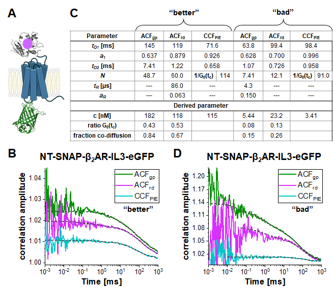
Figure 5: Double-labeled NT-SNAP-β2AR-IL3-eGFP construct. (A) In the double labeled construct, the eGFP is inserted into the intracellular loop 3 and the SNAP tag attached to the N-terminus of β2AR (NT-SNAP). (B, D) ACFgp, ACFrd and CCFPIE of two measurements of the double-labeled construct. The data is fit to a bimodal two-dimensional diffusion model (eq. 9, CCFPIE) and including additional relaxation terms (eq. 7, ACFgp and ACFrd). The table in panel (C) shows the fit results and the derived parameter concentration (eq. 8), the ratio of the correlation amplitude at zero correlation time (G0(tc)) and the fraction of co-diffusing molecules (eq. 10). Please note that the measurements were acquired on different days, thus slightly different factor for the amplitude correction were used (B: rGR,DNA = 0.51 and rRG,DNA = 0.79; D: rGR,DNA = 0.51 and rRG,DNA = 0.56). Please click here to view a larger version of this figure.
Double-labeled construct undergoing FRET: β2AR-IL3-eGFP-CT-SNAP
In the double-labeled construct β2AR-IL3-eGFP-CT-SNAP (Figure 6A), the eGFP is inserted into the intracellular loop 3 identical to the NT-SNAP-β2AR-IL3-eGFP construct with the SNAP tag attached to the C-terminus. Here, both labels are on the same side of the cells' plasma membrane, so that the fluorophores are in close vicinity so that FRET occurs as indicated by the quenched eGFP lifetime (Supplementary Note 5). Considering the flexibility of relatively unstructured protein regions like the C-terminus34 and at least two different protein conformations of GPCRs35, "high FRET" (HF) or "low FRET" (LF), dynamic changes in the FRET efficiency due to eGFP-SNAP distance changes could be observed and identified by an anticorrelation term in the CCFFRET (orange curve in Figure 6B). FRET fluctuations have been shown to be anticorrelated as the receptor can only be in one state at a time, either HF or LF. Joint (or global) fit of all five correlation curves (Figure 6B) reveals ~70% of slowly diffusing molecules at ~100 ms while the rest diffuses with ~ 1 ms. All autocorrelations and CCFFRET show relaxation terms at 37 µs and 3 µs; those correlations dominated by red signal (ACFrp, ACFrd and CCFFRET) show an additional slow component ~ 50 ms (Figure 6C).
FRET-induced changes on the CCFFRET under different conditions (Figure 6D) are demonstrated by a series of simulations of a two-state system with a fluctuation time of 70 µs between LF and HF states. Upon switching from the LF to the HF state, changes in the anticorrelated signal are observed in the prompt time window: The green signal decreases and the red signal increases (vice versa for the HF -> LF switching). If HF-LF switching occurs on timescales faster than the diffusion time, in other words during the residence time of the molecule in the focus, the rate can be derived from the anticorrelation in the CCFFRET6,31,36. Please note that dynamic processes slower than the diffusion time cannot be observed in FCS.
In this demonstration, two different FRET scenarios were assumed, showing either a moderate or maximal change in FRET efficiency between the two states. The simulations were performed using Burbulator37 and consider absence or presence of triplet blinking and increasing amount of donor crosstalk into the red channels. The diffusion term was modeled as a bimodal distribution with 30% of fast diffusing molecules at tD1 = 1 ms and the rest of the molecules diffusing slowly with tD2 = 100 ms. In total, 107 photons were simulated in a 3D Gaussian-shaped volume with w0 = 0.5 µm and z0 = 1.5 µm, a box size of 20, and NFCS = 0.01.
Figure 6E-F shows the simulation results for the FRET-induced cross-correlation CCFFRET for moderate (Figure 6E) and maximal FRET contrast (Figure 6F) in the absence (solid lines) and presence of triplet blinking (dashed lines). The FRET-induced anti-correlation can easily be seen in Figure 6F. The "dampening" effect upon adding an additional triplet state reduces the correlation amplitude (Figure 6E-F)38,39.
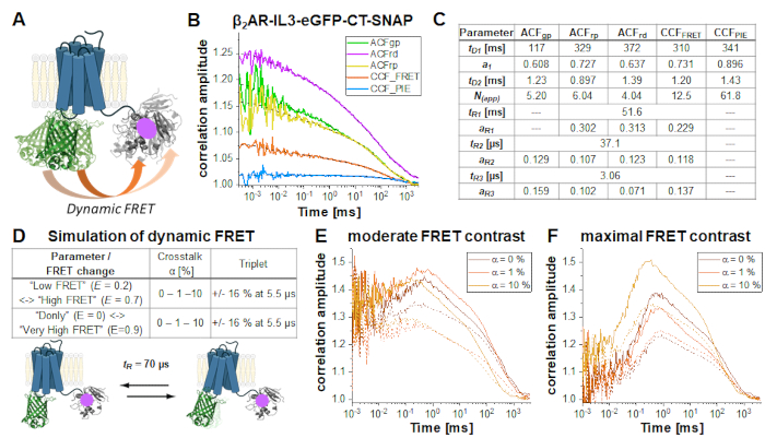
Figure 6: Simulation of double-labeled sample showing dynamic FRET. (A) Double-labeled β2AR with an eGFP inserted into the intracellular loop 3 and a C-terminal SNAP tag. Both fluorophores are close enough to undergo FRET and show changes in the FRET efficiency if the receptor undergoes protein dynamics. (B) Autocorrelation (ACFgp, ACFrp and ACFrd, fit with eq. 7) and cross-correlation curves (CCFFRET (eq. 7) and CCFPIE (eq. 9)) of an example measurement. Table in panel (C) shows the fit results. (D-F) To show the influence of experimental parameter on the expected, FRET-induced anticorrelation term, 12 simulations were performed, in which the change in the FRET efficiency (small or large), different amount of donor crosstalk into the acceptor channels (0%, 1% or 10%) and the absence and presence of triplet blinking were modeled. The equilibrium fraction of both FRET-states was assumed to 50:50 and their exchange rates adjusted such that the obtained relaxation time tR = 70 µs. More details on the simulations see in the text. (E) CCFFRET of the simulation results with a moderate FRET contrast and in the absence of crosstalk (dark orange), 1% crosstalk (orange) and 10% crosstalk (light orange). Solid lines show results in the absence of triplet, dashed lines in the presence of triplet. (F) CCFFRET of the simulation results with maximal FRET contrast. The color code is identical to (E). Please click here to view a larger version of this figure.
However, in the simulation most similar to the experimental conditions (α = 10%, 15% triplet blinking and moderate FRET contrast, dashed yellow line in Figure 6E), the anticorrelation term is nearly diminished. Figure 7 shows the result of analyzing this simulated data using the information encoded in the photon arrival time histograms (i.e., the fluorescence lifetime) by means of Fluorescence Lifetime Correlation Spectroscopy (FLCS)17,19 or species-filtered FCS (fFCS)18. Here, the fluorescence lifetimes of the known HF and LF species (Figure 7A) are used to generate weights or "filters" (Figure 7B) which are applied during the correlation procedure. In the obtained species-auto- and cross-correlation curves (Figure 7C-D) the anticorrelation can be clearly observed.
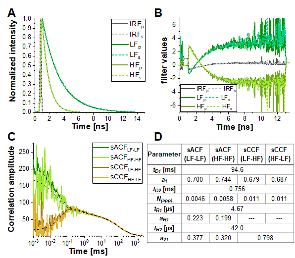
Figure 7: Lifetime-filtered FCS can help to uncover the protein dynamics based fluctuations in FRET efficiency in samples with high crosstalk, significant triplet blinking or other photophysical or experimental properties masking the FRET-induced anticorrelation in the CCFFRET. Here, the approach is shown exemplary for the data shown in Figure 6E for the simulation containing 10% crosstalk and 5% triplet blinking. (A) Normalized fluorescence intensity decay patterns for the two FRET-species (light and dark green for high and low FRET, respectively) and the IRF (grey). The pattern for the parallel detection channel is shown in solid lines, dashed lines for the perpendicular detection channel. (B) The weighting function or "filter" were generated based on the patterns shown in (A), color code is identical to (A). Please note that only the signal in the green detection channels, and thus the FRET-induced donor quenching, is considered here. (C) Four different species-selective correlations are obtained: species-autocorrelations of the low FRET state (sACFLF-LF, dark green) and the high FRET state (sACFHF-HF, light green), and the two species-crosscorrelations between the low FRET to the high FRET state (sCCFLF-HF, dark orange) and vice versa (sCCFHF-LF, orange). The sCCF clearly shows the anticorrelation in the µs-range. Dashed black lines show the fits. sACF were fit with eq. 9 and sCCF with eq. 11. Table in panel (D) shows the fit results. Please click here to view a larger version of this figure.
CCFPIE amplitude to study Protein-Protein Interaction (PPI)
Finally, a common use case for PIE-based FCS in live cells is to study the interaction between two different proteins. Here, the read-out parameter is the amplitude of the CCFPIE, or more precisely the ratio of the autocorrelation amplitudes ACFgp and ACFrd to the amplitude of CCFPIE. To show the effect of increasing co-diffusion on CCFPIE, simulations have been performed based on the two single-labeled constructs, β2AR-IL3-eGFP and NT-SNAP-β2AR (Figure 8A). Figure 8B shows how the amplitude of CCFPIE increases when the fraction of co-diffusing molecules changes from 0% to 100%. Please note that a 1% crosstalk of green signal into the red channels in the delay time window was added with the diffusion components otherwise modeled as shown above.
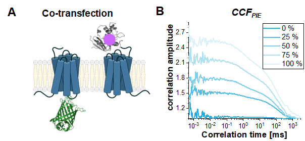
Figure 8: The CCFPIE can be used to study the interaction of two proteins. (A) Here, a co-transfection study of β2AR-IL3-eGFP with NT-SNAP-β2AR (carrying a "red" SNAP-label) was simulated. (B) For an increasing amount of co-diffusing molecules (0% (dark blue) -> 100% (light blue)) the amplitude G(tc) increases. The diffusion term was again modeled as a bimodal distribution with 30% of fast diffusing molecules at tD1 = 1 ms and the rest of the molecules diffusing slowly with tD2 = 100 ms. Additionally, 1% crosstalk of green signal into the red delay time window was added. Please click here to view a larger version of this figure.
| Symbol | Meaning (common unit) | |||
| α | crosstalk of the green fluorophore after green excitation into the red detection channels (%) | |||
| a1 | fraction of first diffusion component in bimodal diffusion model of membrane receptors | |||
| af | total amplitude of the anticorrelation term | |||
| aR | amplitude of photophysics /triplet blinking | |||
| b | baseline / offset of a correlation curve | |||
| B | molecular brightness of a fluorophore ((kilo-)counts per molecule and second) | |||
| BG | background (e.g. from an appropriate reference sample: ddH2O, buffer, untransfected cell etc.) | |||
| c | concentration | |||
| CR | count rate (KHz or (kilo-) counts per second) | |||
| δ | direct excitation of the red fluorophore after green excitation (%) | |||
| D | diffusion coefficient (µm²/s) | |||
| G(tc) | correlation function | |||
| N | number of molecules in focus | |||
| NA | Avogadro’s number (6.022*1023 Mol-1) | |||
| rGR, rRG | amplitude ratio of green or red autocorrelation function to the PIE-based cross-correlation function | |||
| s | shape factor of confocal volume element | |||
| tc | correlation time (usually in millisecond) | |||
| tD | diffusion time (usually in millisecond or microsecond) | |||
| tR | relaxation time of photophysics (usually in microsecond) | |||
| tT | relaxation time of triplet blinking (usually in microsecond) | |||
| w0 | half-width of confocal volume element (µm) | |||
| z0 | half-height of confocal volume element (µm) | |||
Table 1: List of variables and abbreviations. For the use of symbols and definition in fluorescence and FRET experiments, the guidelines of the FRET community40 are recommended.
SUPPLEMENTARY FILES:
SuppNote1_Coverslip cleaning.docx Please click here to download this File.
SuppNote2_Confocal Setup.docx Please click here to download this File.
SuppNote3_Data export.docx Please click here to download this File.
SuppNote4_FCCS calibration analysis using ChiSurf.docx Please click here to download this File.
SuppNote5_Fluorescence lifetime histograms.docx Please click here to download this File.
S6_Scripts.zip Please click here to download this File.
S7_Excel_templates.zip Please click here to download this File.