Learning Objectives

Animals and optical stimulation
Experiments are performed on houseflies (Musca domestica) obtained from a culture maintained by the Department of Evolutionary Genetics at the University of Groningen. Before the measurements, a fly is immobilized by gluing it with a low-melting-point wax in a well-fitting tube. The fly is subsequently mounted on the stage of a motorized goniometer. The center of the two rotary stages coincides with the focal point of a microscopic setup²⁴. The epi-illumination light beam is supplied by a light source, which focuses light on a diaphragm that is imaged at the fly's eye via a half-mirror. It, thus, activates the pupil mechanism of a restricted set of photoreceptor cells (Figure 3). The optical axes of the ommatidia that harbor these photoreceptors are assessed by rotating the fly in small steps and taking photographs after each step with a color digital camera attached to a microscope (Figure 2). Because the pupillary pigment granules reflect predominantly in the long-wavelength range, the red channel of the digital camera is used to discriminate the pseudopupil from the facet lens reflections. The latter reflections are best isolated from the pseudopupil using the camera's blue channel.

Autofocusing and autocentering algorithms
The main additional algorithms used while scanning an insect's eye are the autofocusing and autocentering (Supplementary File 1, scripts AF and AC). The goal of autofocusing is to bring the corneal level to the focus of the camera, in order to detect the facet reflections that are necessary for the identification of individual ommatidia (Figure 3B). The procedure for detecting the corneal level is to change the vertical (Z) position of the fly in steps by applying the fast Fourier transform (FFT) to the image taken at each level to determine the spatial frequency content. The criterion for optimal focus is the level with the greatest summed power above a low-frequency cutoff.

The inputs for autofocusing are the Z-positions and streaming video from the camera. The outputs are the integral of the high-frequency content of the image SF and the focusing level Z where SF is maximal. In the initial step, the Z-position of the camera image is adjusted to slightly below the corneal facet lenses, and the region of interest to determine the image's frequency content is set. The for loop starts the image capture and calculates the sum of the high-pass filtered Fourier-transform SF. By then stepping the z-axis motor upward to an image level above the cornea, the level with the highest frequencies is found, i.e., where SF is maximal, which is taken to be the corneal level. The z-axis motor is then adjusted to that level and an image is taken.

When focusing down from the cornea toward the level of the eye's center of curvature, the corneal facet reflections fade away, and the pseudopupil reflections coalesce into a typical seven-dot pattern, which is a characteristic for the organization of the photoreceptors within the fly ommatidia (Figure 3C; note that the pattern is only distinct in approximately spherical eye areas). The pattern at the eye's center of curvature level is called the deep pseudopupil (DPP)^19,21.

Shifting the fly positioned at the stage with the X- and Y-motors so that the center of the light spot coincides with the center of the camera image is called autocentering. This procedure aligns the facet of the ommatidium whose visual axis is in the center of the DPP with the illumination beam and the optical axis of the microscope and camera. The image is Gaussian filtered and binarized, and then the center of the pseudopupil is determined using the regionprops MATLAB function. The inputs are the positions of the X- and Y-motors and the streaming video from the camera; the output is the distance between the centers of image and pseudopupil, which is then translated into a stage shift.

Correlating images
The eye is scanned by taking and storing photographs at various values of the goniometer elevation θ and azimuth φ after the autofocusing and autocentering procedures. Two-dimensional correlation is used to determine the x-y shifts between successive images. To correlate the images obtained at different angular positions, it is essential to realize that this generally results in a rotation of the current image with respect to the previous image. For instance, let us assume that the center of an initial image corresponds to point C of a sphere (Figure 5) and that a change in azimuth occurs so that plane OAB is rotated over a small angle Δφ, becoming plane OA'B. The center of the image then changes from point C to point C' (Figure 5). If the camera image plane is perpendicular to the vector OC, rotation of plane OAB to OA'B causes rotation of the image over an angle β = Δφ cosθ, as β = CC'⁄BC, with CC' = CDΔφ, and cosθ = CD⁄BC (Figure 5). This means that at the top of the sphere (θ = 0°), β = Δφ, and at the equator (θ = 90°), β = 0°. When Δφ = 0°, that is, when only the elevation θ is changed, the images are not rotated with respect to each other, so β = 0°.

During the scanning procedure, the autocentering procedure centers the ommatidium whose visual axis is aligned with the optical axis of the measuring system. Rotation of the azimuth causes a rotation by an angle β and a translation of the facet pattern. To determine the latter shift, two successive images are correlated (after first rotating the first image by the rotation angle β), as explained in Figure 6.

In the image shift algorithm (Supplementary File 1, script ImProcFacets), the individual facets are identified by the centroids of their reflections in each image. The inputs to the algorithm are the elevation and azimuth angle, the set of images to be assessed, the image channel, and the region of interest. The algorithm produces a set of centroids and a final image that contains all of the correlated images taken during the scanning procedure.

The goniometric system
In order to achieve alignment with the illumination, the fly's eye has to be photographed with the corneal facet lenses in focus, and the pseudopupil must be recentered frequently (here, after every 5° of rotation). This automatic process is realized with the GRACE system (Goniometric Research Apparatus for Compound Eyes), shown schematically in Figure 4. It consists of three main subsystems: the lower and upper stages with their respective electronics as the electromechanical hardware, the firmware embedded in the physical controllers, and the PC used to operate the software that implements the algorithms. The hardware consists of the motorized and optical stages, the digital camera, a microcontroller for programming LED intensities, and a white LED light source. The firmware's routines are provided with the motor controllers, the LED Controller, and in the digital camera. The software consists of the algorithms for controlling motor positions and speeds, adjusting the LED, and acquiring and analyzing images. The algorithms discussed next represent the major milestones that enable the GRACE system to scan insect eyes.

Fly eyes and pseudopupils
When a housefly eye is illuminated, the incident light activates the pupil mechanism of the photoreceptor cells, a system of mobile, yellow-colored pigment granules inside the cell body. The system controls the light flux that triggers the phototransduction process of the photoreceptors, and thus has essentially the same function as the pupil in the human eye^19,20. The activation of the pupil mechanism causes a locally enhanced reflection in the eye area facing the aperture of the microscope's objective (Figure 3). The position of the brightly reflecting eye area, the pseudopupil^19,20,21, changes upon rotation of the eye because the incident light then activates the pupil mechanism in a different set of photoreceptor cells (see Figure 6). The pseudopupil thus acts as a marker of the visual axis of the ommatidia that are aligned with the microscope. This allows mapping of the spatial distribution of the eye's visual axes ^{4,20,21,22,23}.

Filling in missing facets
Not all facets are identified by the centroid procedure, for instance, due to a low local reflectance caused by minor surface irregularities or specks of dust. The latter can also result in erroneous centroids (Figure 7A). This problem is resolved first by washing the eyes under a water tap and secondly by applying a filling-in procedure (script ImProcFacets). Therefore, the centroids in an area are first determined (Figure 7A), and then the FFT is calculated (Figure 7B). The first ring of harmonics (yellow stars in Figure 7B) defines three orientations, indicated by the blue, red, and green lines (Figure 7B). Inverse transformation of the harmonics along the three orientations yields the gray bands in Figure 7C–E. Fitting a second-order polynomial to the gray bands yields lines connecting the facet centroids along the three lattice axes. The crossing points of the lattice lines, thus, correspond to the true facet centers. As the example of Figure 7 is an extreme case, it demonstrates that the procedure is robust. In most areas, missing facets and erroneous centroids are rare.

Scanning a fly eye
Figure 8 shows a band of ommatidia scanned across the eye by performing a series of stepwise azimuthal changes with Δφ = 5°. Scanning from the frontal side of the eye (Figure 8A, right) to the lateral side (Figure 8A, left) occurred in 24 steps. The centroids of the largely overlapping facet patterns were subsequently rotated by β = Δφcosθ. Then, after shifting the centroids of each image and filling in the missing facets (with script ImProcFacets), the colocalized centroids were averaged. Figure 8A shows the combined images, together with the image centers and facet centroids. Figure 8B shows the assembly of facets as a Voronoi diagram.

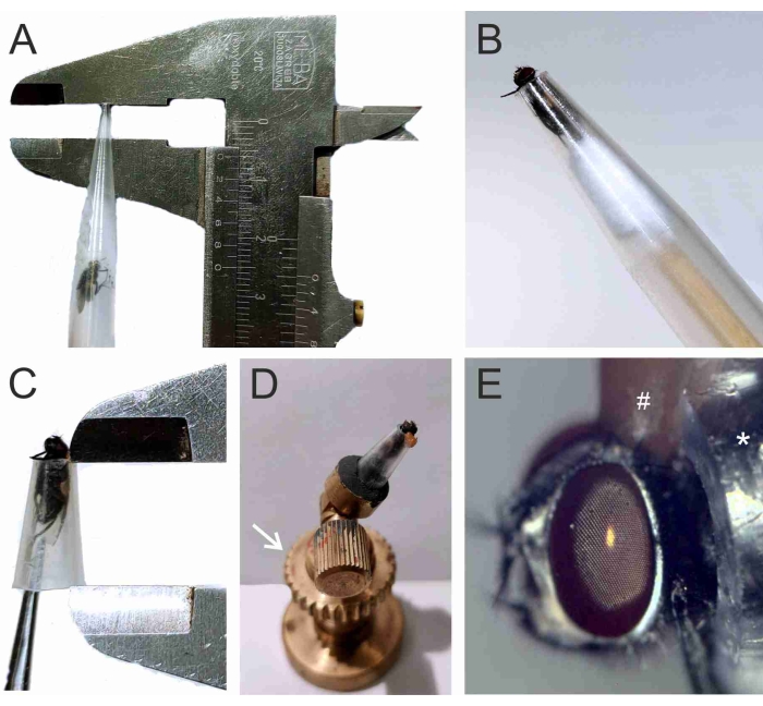
Figure 1: Mounting the fly into the brass holder. (A) A tip with a housefly to be investigated. (B) The cut tip with the fly gently pushed to the end using a piece of cotton and a chopstick. (C) The tip with the fly further cut to a total length of 10 mm. (D) The brass holder with the fly to be placed on the goniometer stage; the arrow points to the height adjustment screw. (E) Close-up photo of the fly with the head immobilized by a piece of low-temperature melting wax (#) to the tip (*). Epi-illumination has activated the pupil mechanism of the eye's photoreceptors, as revealed by the yellow pseudopupil. Please click here to view a larger version of this figure.

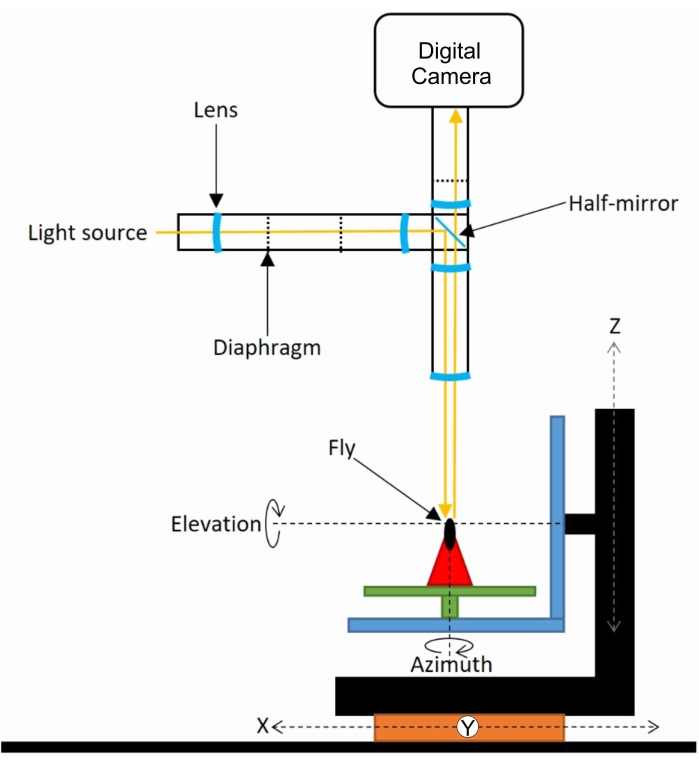
Figure 2: GRACE, the Goniometric Research Apparatus for Compound Eyes. The investigated insect (a fly) is mounted at the motorized stage consisting of three translation stages (X, Y, Z) and two rotation stages (elevation and azimuth). A lens focuses light from a white LED at a diaphragm, focused via a half-mirror at the fly's eye. The eye is photographed with a camera attached to a microscope. Please click here to view a larger version of this figure.

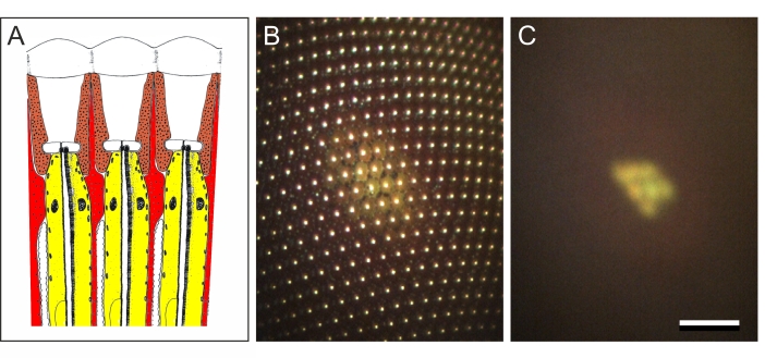
Figure 3: Optics of fly eyes. (A) Diagram of three ommatidia of a fly eye, each capped by a biconvex facet lens, which focuses incident light onto a set of photoreceptor cells (yellow), surrounded by primary (brown) and secondary (red) pigment cells. Intense illumination of dark-adapted (DA) photoreceptors causes migration of yellow pigment granules (indicated by black dots), which exist inside the photoreceptor cells. Accumulated toward the tip of the photoreceptors, near the light-sensitive organelles, the rhabdomeres, they absorb and backscatter light in the light-adapted (LA) state. (B) Image at the level of the eye surface, showing the facet reflections (bright dots) as well as the pigment granule reflection in the activated state (the corneal pseudopupil, CPP). (C) Image taken at the level of the center of eye curvature (the deep pseudopupil, DPP), reflecting the arrangement of the photoreceptor cells in a trapezoidal pattern, with their distal ends positioned at about the focal plane of the facet lenses. A superimposed virtual image of the photoreceptor tips, thus, exists in the plane of the center of eye curvature. Scale bar 100 µm applies to panels B and C. Please click here to view a larger version of this figure.

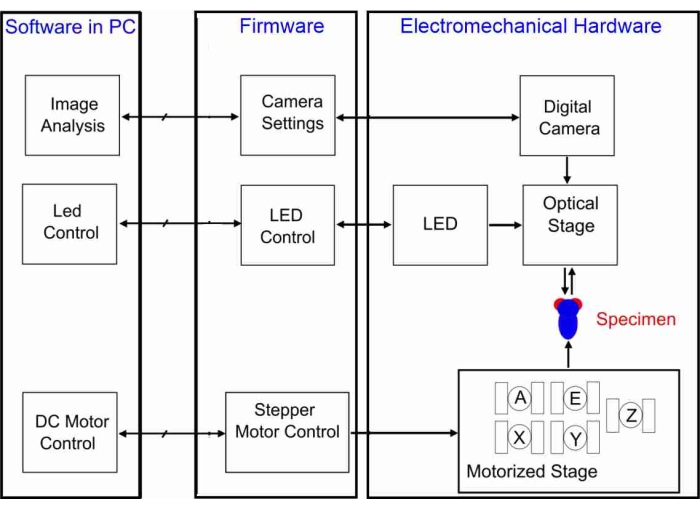
Figure 4: Schematic diagram of the GRACE system. The PC software controls the firmware, which drives the electromechanical hardware. The digital camera takes, via an optical stage, images of the specimen's eye. The LED light source illuminates the specimen, and the motors of the motorized stage actuate the X-, Y-, and Z-translations as well as the azimuth (A) and elevation (E) rotations. Please click here to view a larger version of this figure.

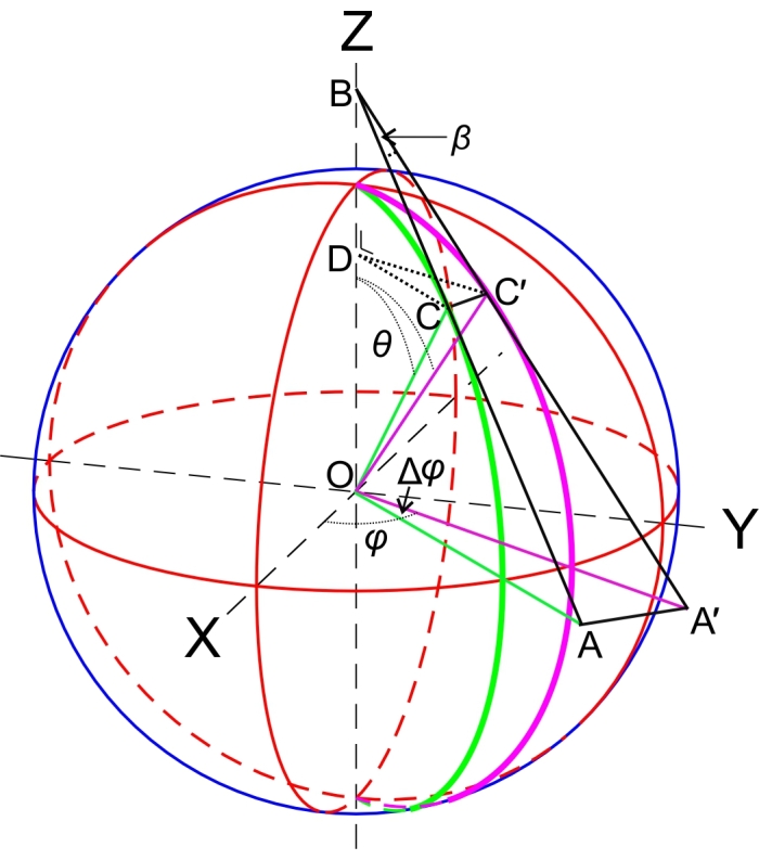
Figure 5: Diagram for deriving the image rotation when scanning the fly eye. If the center of an initial image corresponds to point C of a sphere and a change in azimuth occurs, plane OAB is rotated over a small angle Δφ, becoming plane OA'B. The center of the image then changes from point C to point C'. Rotation of plane OAB to OA'B causes rotation of the image over an angle β = Δφ cosθ (see text, section Correlating images). Please click here to view a larger version of this figure.

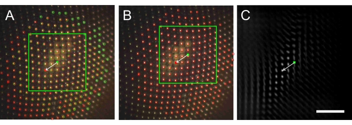
Figure 6: The image processing procedure for determining the interommatidial angle. (A) Image taken during a scan across the eye, with facet centroids marked by green circles and red squares, and a green dot at the image center. (B) Subsequent image after an azimuthal rotation of 5°, with facet centroids marked by red squares and a red dot at the image center. (C) Correlogram of the area within the green square of A correlated with image B. The vector from the center of C (green dot) to the maximum value of the correlogram represents the relative shift of images A and B. Using that vector, the shifted square of A and its center are drawn in B and the facet centroids (red squares) of B are added in A. Scale bar 100 μm applies to panels A-C. Please click here to view a larger version of this figure.

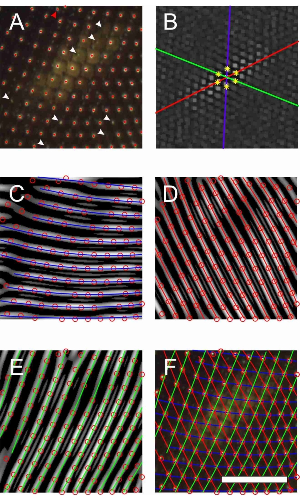
Figure 7: Deriving missing facet centroids by applying Fourier transforms. (A) A local RGB image with facet centroids (red dots). White arrowheads indicate missing facets, and the red arrowhead points to an erroneous centroid. (B) FFT of the centroids of A with the first ring of harmonics marked by yellow stars. (C–E) Inverse FFT of the centroids along the three directions indicated by the colored lines in B, yielding the grayish bands. The blue (C), red (D) and green (E) lines are quadratic polynomial fits to the gray bands, and the centroids (red circles) are those which were obtained prior to the Fourier transforms. (F) The fitted lines of C-E combined, together with the centroids of A. The missing facet centroids are then derived from the crossing points. Scale bar 100 μm applies to panels A, C-F. Please click here to view a larger version of this figure.

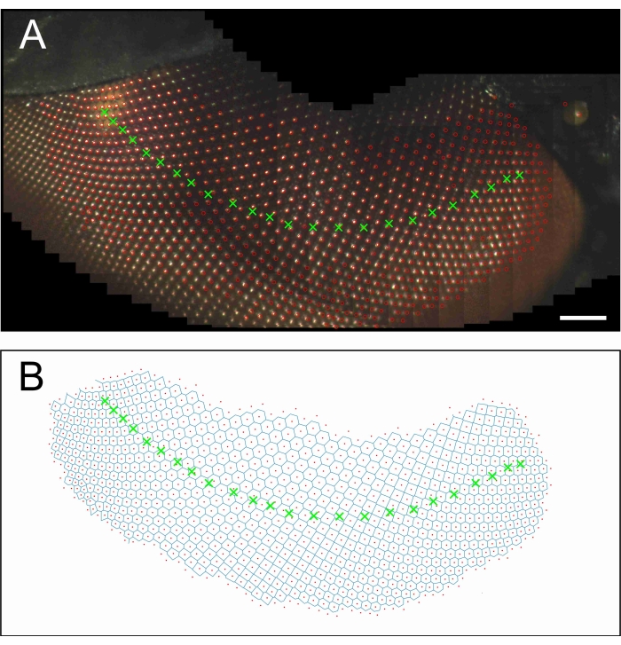
Figure 8: The right eye of a housefly scanned from one side to the other side. (A) Combined, overlapping images of an image series in which the azimuth was changed stepwise by 5°, together with the image centers (green crosses) and the facet centroids (red circles). (B) Voronoi diagram of the facet centroids, with the image centers as in A. Scale bar 100 μm applies to panels A and B. Please click here to view a larger version of this figure.

Supplementary File 1: Please click here to download this File.