All animal studies were approved by the Institutional Animal Care and Use Committee at Northern Arizona University. Extensor digitorum longus (EDL) muscles from male and female wild-type mice (strain B6C3Fe a/a-Ttnmdm/J), aged 60-280 days, were used for the present study. The animals were obtained from a commercial source (see Table of Materials), and established in a colony at Northern Arizona University.
1. Selecting in vivo strain trajectory and preparing for use during ex vivo work loop experiments
NOTE: In this protocol, prior measurements from in vivo dynamic locomotion, provided directly to the authors (Nicolai Konow, UMass Lowell, personal communication), were used in ex vivo experiments. The original data was collected for Wakeling et al.15. Time, length or strain, EMG/activation, and force data are required to replicate the protocol.
- Segment the entire in vivo trial into individual strides using any programming platform (MATLab code provided in Suplementary Coding File 1).
- Plot the length changes vs. time for the entire in vivo trial. This is used to visualize individual strides (stance to stance) and to assess among-stride variability (Figure 1).
- Calculate strain for the entire trial (Length (L) /Maximum Isometric Force at Optimal Length L0).
- Select a stride from the entire trial that is representative of all strides, and that begins and ends at similar lengths. This can be done visually by graphing the lengths on top of each other to compare each stride.
- After a representative stride is selected, segment out strain, EMG/activation, and force data from the entire trial using any programming platform (see Supplementary Coding File 1 for the codes used in MATLab16).
- If sampling frequency differs for strain, EMG/activation or force, interpolate the data points so that all are sampled at the same frequency.
NOTE: Researchers can determine the frequency of capture based on the time intervals between each point sampled in the entire trial. If variables are captured at the same frequency, the sampling times will be the same.
- Calculate the frequency of segmented strides.
- Calculate the frequency by determining the duration of a segmented stride in seconds and dividing 1 (second) by the duration (1/duration = # strides per second).
- Manually determine how many data points must be acquired in ex vivo experiments to match the frequency.
- Calculate the time required for two strides. Repeat the strides at least once for estimating within muscle measurement error, which will be required for subsequent statistical analysis.
- Determine the phase of stimulation relative to strain input using the measured EMG activity to determine the onset and duration of the stimulation for the ex vivo work loops. Any programming platform can be used (see Supplementary Coding File 1 for the code used in this study).
- View EMG signal over the same x-axis range (time) as strain change (Figure 1). Enlarge the EMG signal to be visible; this can be done by multiplying the EMG signal by an arbitrary number, rescaling the strain and EMG to be on the same scale, and/or adding the EMG signal to the strain.
NOTE: Authors rescaled the strain and EMG to be on the same scale using "rescale" function in MATLab (see Supplementary Figure 1). - Find where EMG activity starts and stops, as indicated by a change in intensity of two standard deviations17,18.
NOTE: Depending on the animal and muscle, EMG onset might or might not correspond with foot contact (Monica Daley, UC Irvine, personal communication) (see Discussion section). - Calculate the percentage of the strain cycle (e.g., 40%) at which the EMG activation onset occurs and for how long the stimulation will occur (e.g., 222 ms).
NOTE: Researchers will need to account for an excitation-contraction coupling (ECC) delay that differs between in vivo movement and ex vivo work loops and may be different for each animal and muscle (e.g., in vivo ECC is 24.5 ms for rat MG, ex vivo ECC is ~5 ms for mouse EDL).
- View EMG signal over the same x-axis range (time) as strain change (Figure 1). Enlarge the EMG signal to be visible; this can be done by multiplying the EMG signal by an arbitrary number, rescaling the strain and EMG to be on the same scale, and/or adding the EMG signal to the strain.
- Prepare representative strain inputs for the work loop controller program. Any program that can capture force output with input for strain and stimulation can be used for the work loop controller program (see Discussion section).
- Take the selected stride and interpolate to the appropriate number of points necessary to have the step captured at in vivo frequency for two cycles (see step 1.2).
- Rescale the stride to start and stop at "zero strain" (e.g., L0 or 95% L0) after stretching by a pre-determined length excursion (see step 3.3).
- "Scale" selected stride, if necessary, to use as an input for strain changes in mouse EDL (see Discussion section). To scale, select a length excursion to which the mouse EDL can be stretched without damage (e.g., we typically stretch the mouse EDL by 10% L0 regardless of the in vivo species). This may need to change based on preliminary results (see step 3.3).
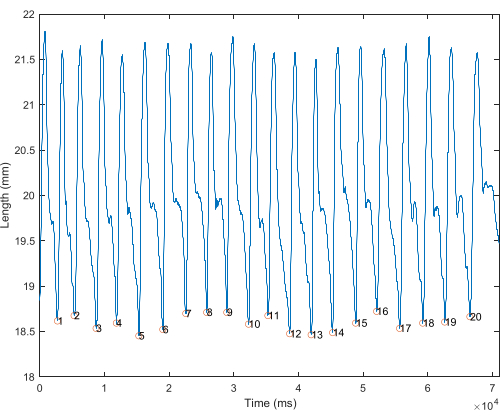
Figure 1: Length over time of in vivo whole trial. Length (mm) plotted against time of rat MG. Strides are demarcated by circles, from shortest length to shortest length, considered single stride. Please click here to view a larger version of this figure.
2. Evaluating maximum isometric force of mouse muscle ex vivo
- Set up equipment and surgery.
NOTE: See the Discussion section for an explanation of the equipment needed for the ex vivo work loop.- Prepare a tissue-organ bath by inserting the oxytube needle valve into the water-jacket tissue bath (see Table of Materials). Connect the oxytube to a gas cylinder with 95% 02-5% CO2. Allow 20 psi to fill the water-jacket tissue bath.
- Prepare the surgery area by running an additional oxytube from the gas line to a crystallizing dish filled with Krebs-Henseleit solution (step 2.1.3) near the surgery area. This will be used to keep the muscles aerated and hydrated during and after the surgeries.
NOTE: Muscles can also be stored in this aerated solution up to 4 h, if more than one muscle is taken out of the mouse at a time. - Prepare 1 L of Krebs-Henseleit solution containing (in mmol l-1): NaCl (118); KCl (4.75); MgSO4 (1.18); KH2PO4 (1.18); CaCl2 (2.54); and glucose (10.0) at room temperature and pH to 7.4 using HCl and NaOH (see Table of Materials). When handling HCl and NaOH, wear the proper PPE of goggles and gloves.
- Fill the bath with Krebs-Henseleit solution at room temperature and pH 7.4. Submerge the muscle and the hook completely in the solution.
- Turn on all equipment; dual-mode muscle lever system, stimulator, and signal interface (DAQ board) (see Table of Materials).
- EDL muscle dissection.
- Deeply anesthetize the mouse and then perform euthanasia by cervical dislocation. Lay the mouse in either a right or left lateral recumbent position with the top hindlimb stretched and toes touching the dissection board. Remove the fur from the ankle to above the knee joint.
- Tent the skin with forceps and cut from the ankle joint to the hip area. Once the muscle has been exposed, cut around the ankle like a "hem" of pants. Pull the skin up to expose the leg muscles more clearly.
- Locate the fascia line that separates the tibialis anterior (TA) and gastrocnemius, separate using dissection scissors to expose the knee tendons. Place dissection scissors between the two exposed knee tendons. Scissors will "catch" on a pocket just below the exposed knee tendons. Blunt dissect a "pocket" while pulling the scissors away from the leg until the scissors reach the ankle to expose the EDL.
- Using a pre-tied loop knot in size 4-0 silk surgical suture (see Table of Materials), lace one end of the suture under the tendon closest to the knee. Tie a double square knot above the proximal muscle-tendon junction without placing it on the muscle or including the tendon. Cut above the knot. Gently pull the loop tied to the tendon, and the EDL will emerge from the "pocket".
- Tape the loop to the dissection area to create tension in the EDL. Tie a double square knot using another pre-tied loop knot at the distal muscle-tendon junction without placing it on the muscle or including the tendon. Cut the knot on the side closer to the leg to remove the whole EDL from the mouse. Cut the extra suture away from the double square knots on the proximal and distal sides of the muscle and place the muscle in the aerated bath by the surgery area.
NOTE: Ensure to note which side is proximal and/or distal if placing the muscle in an aerated bath. - To place on the servomotor lever rig, attach EDL vertically between suspended platinum electrodes. Attach the distal loop knot to the stationary hook and attach the proximal loop knot to the hook attached to the servomotor arm. Raise the tissue bath to submerge the muscle in the aerated Krebs-Henseleit solution.
NOTE: Aeration should not disturb the muscle when it is submerged. If it does, lower the pressure of the gas. Allow muscle to equilibrate for 10 minutes before beginning stimulation.
- Measure the maximum isometric force of EDL muscle.
NOTE: Refer to Table 1 for protocol on how to measure maximum isometric force using twitch and tetanus. See Supplementary Figure 1 for an illustration of the program used by the authors.- Stimulate the muscle with a supramaximal twitch to ensure the muscle has not been damaged during surgery (80 V, 1 pps, 1ms; Table 1; see Supplementary Figure 2). If no damage has occurred, use the length knob on the muscle lever system to find a muscle length using twitch stimulation at which active tension is ~1V / 0.1271 N with less than ~0.1V / 0.01271N passive tension.
- Record the starting length of the muscle from suture knot to suture knot in Volts and millimeters. Input measurements into the calibration portion of the program for starting length (see Supplementary Figure 1).
- Find supramaximal twitch maximum isometric force at optimal length (L0) of EDL (Table 1). No rest period is technically needed, but waiting 1 min between stimulations will stabilize passive tension. Record the length (in Volts) at which the supramaximal twitch is maximum. This is the muscle optimum length (L0) for twitch.
- Measure the muscle with calipers at this length. Measure the muscle from suture knot to suture knot. Once L0 has been found, shorten the muscle back to starting length (active tension ~1V / 0.1271 N).
- Find supramaximal tetanus maximum isometric force of EDL (80 V, 180 pps, 500 ms; Table 1). Record the length (in Volts and millimeters) of supramaximal tetanic force at L0 and measure the fibers from suture knot to suture knot again with calipers.
NOTE: Increasing the muscle length in 0.5 V/0.65 mm steps will result in more accurate L0 for both twitch and tetanus. - Find the submaximal isometric force of EDL (45 V, 110 pps, 500ms; Table 1) at L0 before and after the experiment to ensure fatigue did not occur from the stimulation protocol. A 10% decrease in force is considered a "fatigued" muscle.
| Experiment | Simulation Intensity (V) | Pulse Frequency (pps / Hz) | Stimulation Duration (ms) | Comments | ||||||||
| 1. "Warm-Up" | 80 | 1 | 1 | Increase or decrease length by 0.50 V to find passive tension of 1 V | ||||||||
| 2. Optimal muscle length twitch (L0) | 80 | 1 | 1 | Increase or decrease length by 0.50 V to find passive tension of ~1 V | ||||||||
| 3. Optimal muscle length tetanus (L0) | 80 | 180 | 500 | Rest 3 min between changing length by 0.50 V | ||||||||
| 4. Pre-experiment submaximal L0 | 45 | 110 | 500 | At length of L0 | ||||||||
| 6. Avatar experiments | 45 | 110 | Cyclically use representative length changes for mouse EDL | |||||||||
| 7. Post-experiment submaximal L0 | 45 | 110 | 500 | Return to L0 after experiment and measure L0 | ||||||||
Table 1: Stimulation protocol. Stimulation protocol for finding supramaximal and submaximal twitch and tetanus optimal length. Protocol varies by stimulation intensity, timing, and pulses per second.
3. Completing "avatar" work loop technique using selected in vivo strain trajectories
- Set up the software necessary to complete "avatar" work loop techniques (see Table of Materials).
NOTE: An input file (.csv or similar) that specifies the muscle length at each time step is needed (see step 1.4). Inputs for the percentage of the cycle at which the stimulation starts and for the duration of stimulation are necessary (see Supplementary Figure 3 for example). - Complete "avatar" work loop technique.
NOTE: While we use a custom LabView program, researchers can use any program that allows control of length changes in mouse EDL on a servomotor lever, control of the onset (% cycle) and duration (ms) of stimulation at specified times, and measurement of muscle force. See Supplementary Figure 3 for an illustration of the program authors use.- Upload the scaled strain changes with scaled length excursion into the program from step 1.4. See steps 1.4, 3.3, and the Discussion section for more on "scaled strain changes".
- Adjust the starting length of the muscle if needed (see section 3.3). Input the starting length in V and mm to calibrate results (see Supplementary Figure 3).
- Use stimulation onset and duration calculated in step 1.3.
- Run the muscle through the scaled length changes with determined length excursion for two cycles.
- Save data. If several stimulation protocols are collected on the same muscle, wait 3 min between each stimulation.
- Stimulate at optimal length (L0) using submaximal activation to determine if fatigue has occurred. If force decreases by more than 10%, muscles are considered fatigued. See Table 1 for stimulation protocols.
- Remove the muscle from the bath. Cut-loop knots from the muscle and dab the excess solution off the muscle. Weigh the muscle. Determine physiological cross-sectional area using the standard formula: muscle mass/(L0*1.06)19.
- Tune parameters for "avatar" work loop technique (see Discussion section).
- Determine the starting length and length excursion by matching the ex vivo passive tension rise to the passive tension rise observed in vivo (Figure 2).
NOTE: This study used percent L0 to scale starting length (mm) and excursion (% L0; see step 1.4 and Discussion section). For matching the tension rise in ex vivo mouse EDL to that of the in vivo rat MG, the authors found that starting length at L0 produced the best fit (Figure 2). - Choose three starting lengths (e.g., -5% L0, L0, and +5% L0). Perform the "avatar" work loop at each of these starting lengths with a specified length excursion (e.g., 10% L0).
NOTE: In the present "avatar" experiments using mouse EDL, a length excursion of 10% L0 was used. - Repeat with new starting lengths and/or excursion until the rate of ex vivo passive tension rise is similar to the rate of in vivo passive tension rise (see Figure 2B).
- Depending on fiber types and activation dynamics of the muscles used, increase or decrease the duration of stimulation to optimize the match between ex vivo and in vivo force. Thus, it may be necessary to change the onset and/or duration of stimulation to best match in vivo force production during "avatar" experiments.
- To decide whether this is necessary (see Discussion section), plot force over time of "avatar" and in vivo muscle (Figure 3) and calculate the coefficient of determination R2 by squaring the scaled correlation between target and "avatar" muscle force (see Representative results).
- Determine the starting length and length excursion by matching the ex vivo passive tension rise to the passive tension rise observed in vivo (Figure 2).
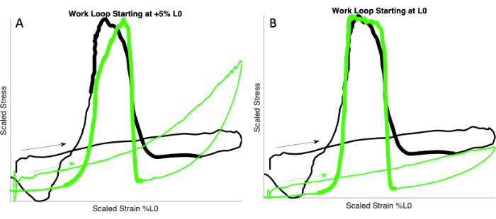
Figure 2: Matching passive tension rise. Work loops showing the in vivo and ex vivo rise in passive tension (arrows). In vivo scaled work loop from rat MG (black) walking at 2.9 Hz (data from Wakeling et al.15). Ex vivo scaled work loops from mouse EDL (green) at 2.9 Hz. (A) Starting length of mouse EDL muscle is +5% L0. (B) Starting length of the mouse EDL muscle is L0. Note that the ex vivo passive tension rise matches the in vivo tension rise in A but not in B. Thicker lines indicate stimulation. Please click here to view a larger version of this figure.
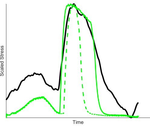
Figure 3: Optimizing stimulation duration of mouse EDL to match in vivo force of rat MG (black line). The force generated by the mouse EDL using the EMG-based stimulation (green dashed line) decreases earlier than the in vivo force, likely due to faster deactivation of the mouse EDL compared to rat MG. To optimize the fit between the in vivo and ex vivo forces, the mouse EDL was stimulated for a longer duration (solid green line). EMG-based stimulation R2 = 0.55, Optimized stimulation R2 = 0.91. Please click here to view a larger version of this figure.
The goal of the "avatar" experiments is to replicate in vivo force production and work output as closely as possible during ex vivo work loop experiments. This study chose to use mouse EDL as an "avatar" for rat MG because mouse EDL and rat MG are both comprised of mostly of fast-twitch muscles20,21. Both muscles are primary movers of the ankle joint (EDL ankle dorsiflexor, MG ankle plantarflexor) with similar pennation angles (mouse EDL 12.4 + 2.12°22, rat MG 20° used in this study15). Scaled representative work loops of rat MG15 were compared to ex vivo "avatar" experiments (Figure 4) using two different stimulation protocols (one from measured EMG activity and one optimized as in step 3.3). R2 values presented here were calculated using the entire scaled stretch-shortening cycle (2 cycles/condition), with each cycle having more than 2000 points corresponding to the locomotor speed (walk = 5521 points, trot = 5002, gallop = 2502 points). Work loops were scaled to account for differences in muscle size, P0, and PCSA. Scaling was done by linearly mapping force and strain onto a similar scale (0-1) to compare rat MG and mouse EDL. Visually, it is apparent that optimizing the stimulation protocol (Figure 4B) to account for different activation dynamics of the mouse EDL and rat MG muscles improves the fit to the in vivo rat MG force compared to the EMG-based activation (see Discussion section). For the mouse EDL, approximately doubling the stimulation duration for slower strain trajectories (walk and trot) increased the R2 by 62% in walking and 109% in trot. For the faster strain trajectory (gallop), increasing stimulation time by half the observed time increased the R2 by 22%.
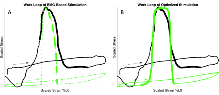
Figure 4: Comparison of in vivo and ex vivo work loops. Work loops of in vivo rat MG (black) and ex vivo mouse EDL (green) during walking (2.9Hz) using in vivo strain trajectories. The thicker line indicates stimulation in both in vivo and ex vivo work loops. (A) Work loop of in vivo rat MG (black) and ex vivo mouse EDL (dashed green) during walking using EMG-based stimulation protocol. (B) Work loop of in vivo rat MG (black) and ex vivo mouse EDL (solid green) during walking (2.9Hz) using optimized stimulation. Please click here to view a larger version of this figure.
High R2 between mouse EDL ex vivo force production and in vivo force production of rat medial gastrocnemius (MG)15 indicates good replication (Figure 5). In EMG-based stimulation experiments, average R2 values were 0.535, 0.428, and 0.77 for walk, trot, and gallop, respectively. In optimized stimulation experiments, average R2 values were 0.872, 0.895, and 0.936 in walk, trot, and gallop, respectively. As previously discussed (step 3.3, Figure 5), depending on the activation dynamics of the muscles used, the stimulation protocol may also need to be optimized. Prediction of in vivo MG force using ex vivo mouse EDL was improved across all locomotor speeds by optimizing stimulation, increasing R2 (Figure 5A,B), and decreasing root mean square error (RMSE). RMSE decreased after optimization for all speeds (Figure 6). Averaged RMSE for EMG-based stimulation was 0.31, 0.43, and 0.158 for walk, trot, and gallop. Averaged RMSE for optimized stimulation was 0.181, 0.116, 0.101 for walk, trot, and gallop.
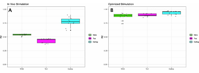
Figure 5: R2 Values for in vivo and ex vivo force production: Box and whisker plot of R2 values for in vivo and ex vivo force comparisons. Individual observations plotted, median, 25th, and 75th percentile indicated. (A) R2 values for in vivo and ex vivo force production using stimulation protocol based on measured in vivo EMG signal during walking at 2.9 Hz (green), trotting at 3.2 Hz (magenta), and galloping at 6.2 Hz (cyan). (B) R2 values for in vivo and ex vivo force production using optimized stimulation (see Figure 2). Optimizing the stimulation onset and duration increased R2 for all gaits. EMG-based stimulation: walk R2 = 0.50-0.55, trot R2 = 0.37-0.47, gallop R2= 0.62-0.90; optimized stimulation: walk R2 = 0.74-0.93, trot R2 = 0.85-0.92, gallop R2 = 0.87-0.97. Please click here to view a larger version of this figure.
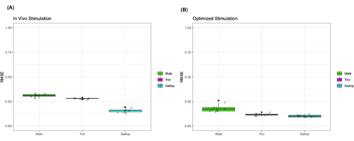
Figure 6: Root-mean square error (RMSE) for in vivo and ex vivo force production. Box and whisker plot of RMSE values for in vivo and ex vivo force comparisons. Individual observations plotted, median, 25th, and 75th percentile indicated. (A) RMSE values for in vivo and ex vivo force production using EMG-based stimulation protocol. (B) RMSE values for in vivo and ex vivo using optimized stimulation protocol. Optimizing the stimulation onset and duration reduced RMSE for all gaits. Walking at 2.9 Hz (green), trot at 3.2 Hz (magenta), and gallop at 6.4 Hz (cyan). Please click here to view a larger version of this figure.
To test the performance of traditional work loop methods at predicting in vivo muscle forces, sinusoidal work loops were also performed for the mouse EDL at the same frequency, length excursion, starting length, stimulation onset, and duration as for the "avatar" experiments using in vivo rat MG strain trajectories. R2 values were significantly lower than for the in vivo strain trajectories for both EMG-based and optimized stimulation protocols (Figure 7). Averaged R2 values for EMG-based stimulation using sinusoidal length trajectories were 0.062, 0.067, and 0.141 at walk, trot, and gallop frequencies. Averaged R2 values for optimized stimulation using sinusoidal length trajectories were 0.09, 0.067, and 0.141 at walk, trot, and gallop frequencies.
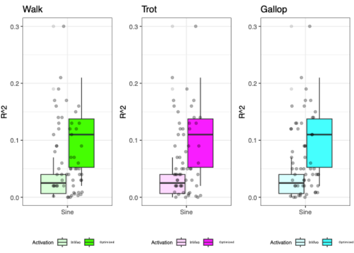
Figure 7: R2 Values for in vivo and ex vivo force production using sinusoidal length changes. Box and whisker plot of RMSE values for in vivo and ex vivo force comparisons. Individual observations plotted, median, 25th, and 75th percentile indicated. R2 values for walk (green, 2.9 Hz), trot (magenta, 3.2 Hz), and gallop (cyan, 6.2 Hz) using sinusoidal length changes with EMG-based (translucent) and optimized (opaque) stimulation protocols. For both EMG-based and optimized stimulation, the R2 values were lower for the sinusoidal length changes than for in vivo length changes. EMG-based stimulation: walk R2 = 0.00 – 0.30, trot R2 = 0.00 – 0.02, gallop R2= 0.03 – 0.07; optimized stimulation: walk R2 = 0.02 – 0.21, trot R2 = 0.02 – 0.12, gallop R2 = 0.12 – 0.17. Please click here to view a larger version of this figure.
Work loops produced by the ex vivo mouse EDL muscle using sinusoidal length trajectories do not as accurately emulate in vivo rat MG force compared to in vivo strain trajectories (Figure 8). The change in work produced by sinusoidal vs. in vivo strain trajectories can be explained by the absence of strain and velocity transients in the sinusoidal trajectory (Figure 9). While the muscles were stimulated at similar lengths during the active shortening phase of the contractions in both sinusoidal trajectories and in vivo-based strain trajectories, the onset of stimulation occurred at different phases of the cycle (e.g., stimulation onset occurred at a phase of 74% for trot EMG-based stimulation, but at a phase of 43% for walking EMG-based stimulation; see Discussion section).
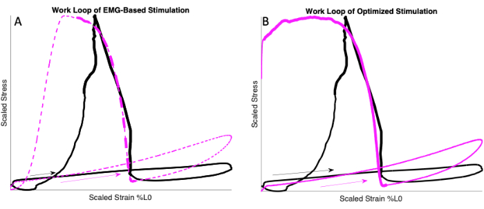
Figure 8: Comparing in vivo and ex vivo sinusoidal work loops. (A) In vivo work loop (black) from rat MG and ex vivo work loop (dashed magenta) from mouse EDL using sinusoidal strain trajectory and EMG-based stimulation. (B) In vivo work loop (black) from rat MG and ex vivo work loop (solid magenta) from mouse EDL using sinusoidal strain trajectory and optimized stimulation. Note that the sinusoidal work loops overestimate the in vivo work due to the absence of strain and velocity transients in the sinusoidal trajectory. EMG-based stimulation R2 = 0.0003, optimized stimulation R2 = 0.084. Please click here to view a larger version of this figure.
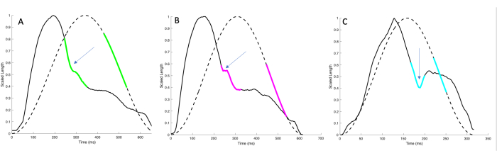
Figure 9: Comparison of in vivo strain and ex vivo sinusoidal length trajectories. Comparison of in vivo strain and ex vivo sinusoidal length trajectories at walk (green), trot (magenta), and gallop (blue). The solid line is in vivo strain trajectory. Dashed line ex vivo sinusoidal length trajectory. The highlighted portion is stimulation. Stimulation started at the same length during the shortening phase of the stride. Arrows indicating strain and velocity transients. Deviations from sinusoidal are impedance from outside forces on muscle. Please click here to view a larger version of this figure.
Supplementary Figure 1: Program used to collect isometric maximal force at optimal length. The program used to determine optimal length during supramaximal and submaximal twitch and tetanic stimulation. Please click here to download this File.
Supplementary Figure 2: Viable twitch response. Twitch response of mouse EDL. Twitch force rises and falls quickly and should reach active tension of ~1 V. "Noise" should be minimal after the peak active tension has been reached. Please click here to download this File.
Supplementary Figure 3: Program used to collect work loop data. The program used to control muscle length of and timing of stimulation in ex vivo work loops. Please click here to download this File.
Supplementary Coding File 1: MATLab code used to segment and create an experimental protocol for the work loop. MATLab code that was used to segment target step information (length, EMG activation, and force) into individual strides. Code includes scaling and interpolating target animal steps into lengths that ex vivo mouse EDL can stretch. Additionally, includes code to smooth EMG signal and compare activation to select onset and duration of stimulation in ex vivo work loop experiments. Please click here to download this File.