Exactly how much does something need to change for a difference to be perceived?
Think of, for instance, young children who grow rapidly—getting taller on a daily basis. However, it’s often difficult to notice subtle changes, especially if they still struggle to reach a basketball.
Over a much longer span, their growth spurt becomes more than perceptible; in fact, the amount can seem enormous! These changes in height are only noticed after a lapse because the small day-to-day differences are too small to be perceivable.
The minimal yet perceived amount is the just-noticeable-difference, which, for this example, is the smallest amount of growth noticed.
This video demonstrates a standard approach for measuring a just-noticeable-difference in shape size. Not only do we discuss the steps required to design and execute an experiment, but we also explain how to analyze the data and interpret the results describing just how small of a change in area is necessary to be perceived.
In this experiment, participants are briefly shown two different circles that vary in size and are forced to choose which one is larger.
During each trial, one is always presented with the same circumference, whereas the other is varied. This approach is referred to as the method of constant stimulus.
In this case, the constant stimulus is designed to have a radius of 10 px and located randomly on either the left or right side of the screen. In contrast, the other circle, called the comparison stimulus, will have a radius that varies between 5 and 9 and between 11 and 15 px.
Given these 10 possibilities, the comparison stimulus is shown 10 times on each side, for a total of 200 trials. The dependent variable is recorded as which stimulus was chosen to be the larger one.
Participants are expected to choose correctly if they perceived a difference in size between the two stimuli. However, when the shapes are closer in circumference and below the just-noticeable difference, performance is predicted to decline.
To begin the experiment, greet the participant in the lab. With them sitting comfortably in front of the computer, explain the task instructions: The screen will have the word “Ready?” on it until they press the space bar.
Watch as two blue stimuli appear and instruct the participant to indicate which stimulus they thought was larger by pressing the ‘L’ key for left- and ‘R’ for right-side responses. Remind them that they should guess if they are not sure which one is larger.
After answering any questions the participant might have, leave the room. Allow them to complete all of the 200 trials over a 5-min period. When they finish, return to the room and thank them for taking part in the experiment.
To analyze the data, first retrieve the programmed output file that captured each participant’s responses. Quickly glance at the data to make sure that performances were sensible—namely, that when the sizes of the comparison stimuli were 5 and 15 px, accuracy was near perfect.
Next, add a column to the output table called ‘Accuracy’ to determine whether the recorded answers are correct or not. Compare those given to the correct responses for all trials. Use the following IF statement to register a 1 when the response given was correct and 0 when it was incorrect.
Now, add another column to the table, labeled ‘Proportion of Comparison Responses’. Compare the column ‘Comparison Position’ with ‘Response’ and use a new IF statement to mark a ‘1’ when the comparison stimulus was chosen or a ‘0’ if the constant circle was chosen.
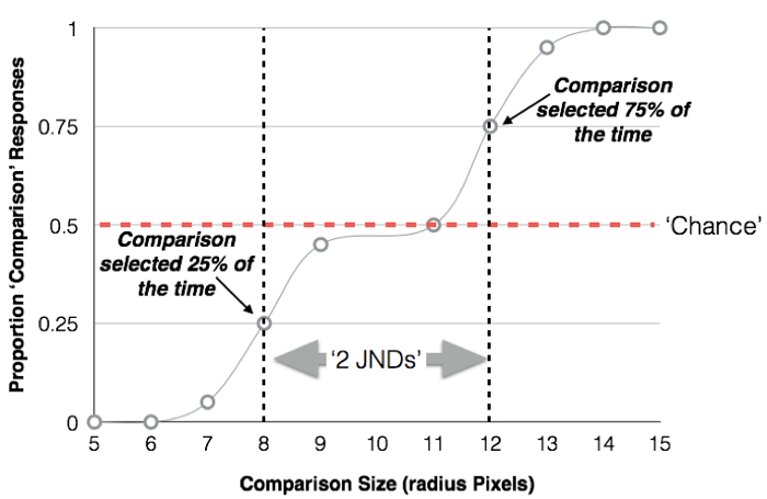
To visualize the results, make a scatter plot with the size of the comparison on the x-axis and the proportion of times it was chosen as being larger on the y-axis. Recall that the constant stimulus always had a 10-px radius, which is why stimuli with 5 or 6 px radii were almost never chosen and those with 14 or 15 were always chosen.
With a radius of 9 or 11 px, the comparison was more difficult and participants often made mistakes. In fact, performance was at chance level, suggesting that differences were not being perceived.
To calculate the just-noticeable-difference, take the comparison size that was chosen 75% of the time, in this case a radius of 12, minus the comparison size that was chosen 25% of the time—radius of 8—and divide the result by 2 for an answer of 2 px.
In other words, the radii of the circles need to differ by at least 2 px for their sizes to be accurately perceived.
Now that you are familiar with just-noticeable differences in the perception of visual objects’ sizes, let’s look at how this paradigm is used in neurophysiological studies to explore how the brain responds and in other behavioral situations, such as distinguishing between fat levels in food.
Researchers have investigated how individual neurons in the visual cortex encode the physical properties of the world, like objects’ sizes.
Using electrophysiological recording techniques that measure firing patterns in conjunction with stimuli presentation, researchers found that neurons that are sensitive to size will sometimes respond in the same way to objects that are actually different sizes.
This is why JND are just-barely-noticeable: sometimes, in the brain, the relevant stimuli really do produce indistinguishable effects.
In addition, researchers have used a just-noticeable-differences task to characterize individual thresholds for detecting fat concentrations in food.
They found that individuals with a higher body mass index required a higher just-noticeable difference, or higher threshold, before tasting fatty acids in the samples. These results could lead to new approaches to limit excess fat consumption.
You’ve just watched JoVE’s introduction to just-noticeable differences. Now you should have a good understanding of how to design and run the experiment, as well as how to analyze and assess the results.
Thanks for watching!