Tree Core Analysis with X-ray Computed Tomography

Summary

Here we show how to process tree cores with an X-ray computed tomography toolchain. Except for chemical extraction for some purposes, no further physical lab treatment is needed. The toolchain can be used for biomass estimations, for obtaining MXD/tree-ring width data as well as for obtaining quantitative wood anatomy data.

Abstract

An X-ray computed tomography (CT) toolchain is presented to obtain tree-ring width (TRW), maximum latewood density (MXD), other density parameters, and quantitative wood anatomy (QWA) data without the need for labor-intensive surface treatment or any physical sample preparation. The focus here is on increment cores and scanning procedures at resolutions ranging from 60 µm down to 4 µm. Three scales are defined at which wood should be looked at: (i) inter-ring scale, (ii) ring scale, i.e., tree-ring analysis and densitometry scale, as well as (iii) anatomical scale, the latter approaching the conventional thin-section quality. Custom-designed sample holders for each of these scales enable high-throughput scanning of multiple increment cores. A series of software routines were specifically developed to efficiently treat three-dimensional X-ray CT images of the tree cores for TRW and densitometry. This work briefly explains the basic principles of CT, which are needed for a proper understanding of the protocol. The protocol is presented for some known species that are commonly used in dendrochronology. The combination of rough density estimates, TRW and MXD data, as well as quantitative anatomy data, allows us to broaden and deepen current analyses for climate reconstructions or tree response, as well as further develop the field of dendroecology/climatology and archeology.

Introduction

Wood density is an easy-to-measure variable¹ that reflects both the anatomical and chemical properties of the wood². In biomass estimations of aboveground biomass, wood density is an important weighing variable ^3,4,5, that is multiplied with the dimensions of the tree and a factor representing the carbon content of the wood. Wood density is tightly linked to the mechanical properties of timber⁶ and reflects the life history of a tree⁷.

Cell wall density is measured as being approximately 1500 kg/m³ and is considered fairly constant⁸, however intra-ring cell wall density variations should be considered as well^8,9.Woody cells (in general tracheids in conifers, vessels, parenchyma and fibers in hardwoods) are oriented/shaped in different ways and cell wall thickness and lumen size of these cells varies¹⁰. Therefore, wood density varies between trees, within a tree (axial and transversal) and within short intervals within a tree ring^11,12. In many cases the wood density variation at the ring scale also delimits the tree ring boundary¹³. Wood density and ultimately tissue fractions are generated and in this paper are broadly put into three categories (i.e., three different resolution scales), depending on the study goal (Figure 1) as described below.

Inter-ring scale: By measuring pieces of wood, a single value is obtained for that sample. This can be done through water immersion or geometrically¹⁴. This way, general biomass or wood technological variables can be obtained. To include pith-to-bark variation, these pieces of wood can be further divided into blocks that are measured manually to obtain information on the life history strategy¹⁵. When switching to low-resolution X-ray CT such as in medical scanners^17,18, TRW data on medium-to-wide rings can be made in an efficient way on many samples^18,19,20. This is also the scale that can be used to assess biomass from pith-to-bark from both temperate and tropical trees^4,22, typically ranging in resolutions from 50 µm to 200 µm.

Ring scale: Wood is a recorder of past environmental conditions. The best known parameter is tree-ring width (TRW), but for global temperature reconstructions, maximum latewood density (MXD) records are proven to be a better proxy for temperature²². MXD is an easy-to-measure variable²³, and a proxy for cell wall thickness and cell size on the last cells of a tree ring, and are at tree line and boreal sites positively linked to seasonal air temperature²⁴: the warmer and longer the summers, more cell wall lignification occurs which thus increases the density of these last cells. Traditional measurements such as immersion and geometry are less accurate to determine this ring-level density. A previous work developed a toolchain for using X-ray film on thin-cut samples²⁵. This sparked a revolution in both forestry and later paleoclimatology^15,18, defining maximum latewood density (MXD), i.e., the peak density value often at the end of a ring, as a proxy for summer temperature. The basic principle is that the samples are sawn (approximately 1.2 mm to 7 mm¹³) to be perfectly parallel to the axial direction, and the sample is put on a sensitive film exposed to an X-ray source. Then these radiography films are read out through a light source that detects the intensity and saves the profiles and the annual tree ring parameters. These tools, however, require a significant amount of sample preparation and manual work. Recently this has been developed for X-ray CT in a more standardized way or based on mounted cores²⁶. Resolution here ranges between 10 µm and 20 µm. TRW is measured on this scale as well, especially when dealing with smaller rings.

Anatomical scale: At this scale (resolution < 4 µm), the average density levels become less relevant as the main anatomical features are visualized and their width and proportions can be measured. Typically, this is done through making microsections or high-resolution optical scans or µ-CT scans. When the ultrastructure of the cell walls needs to be visualized, scanning electron microscopy is the most commonly used method²⁷. At the anatomical scale, the individual tissue fractions become visible so that physiological parameters can be derived from the images. Based on the individual anatomical parameters and the cell wall density of wood, anatomical density can be derived for comparison with conventional estimators of wood density²⁴.

Due to improved sectioning techniques and image software^29,30, dendro-anatomy³⁰ has been developed to have a more accurate record of the wood, both to have a closer estimate of the MXD in conifers and to measure several anatomical variables from broadleaf trees. On this scale, actual anatomical parameters are measured and related to environmental parameters³¹ . With µCT this level can be obtained as well^32,33.

As wood is inherently hygroscopic and anisotropic, wood density needs to be carefully defined and the measurement conditions need to be specified, either as oven-dry, conditioned (typically at 12% moisture content) or green (as felled in the forest)³⁴. For large samples and technical purposes, wood density is defined as the weight divided by its volume at given conditions. However, the value of wood density is strongly dependent on the scale at which it is measured, for instance from pith-to-bark wood density can double, and on a ring scale (in conifers) the transition of earlywood to latewood results in a significant rise in wood density as well, with a peak at the ring boundary.

Here, an X-ray CT scanning protocol of increment cores is presented in order to measure features at the aforenoted 3 scales (Figure 1). Recent developments in X-ray CT can cover most of these scales, due to a flexible set-up. The research goals will determine the eventual protocol for scanning.

A crucial limiting factor (which is inherently connected to the scaled nature of wood density and wood in general) is the resolution and time necessary for scanning. Examples demonstrate how to: (i) obtain inter-ring tree scale wood density profiles for biomass estimations in Terminalia superba from the Congo Basin, (ii) obtain density records from Clanwilliam cedar (Widdringtonia cedarbergensis) based on helical scanning on a HECTOR system³⁵, and (iii) measure vessel parameters on sessile oak, on the Nanowood system. Both scanners are part of the suite of scanners at the UGent Center for X-ray Tomography (UGCT,

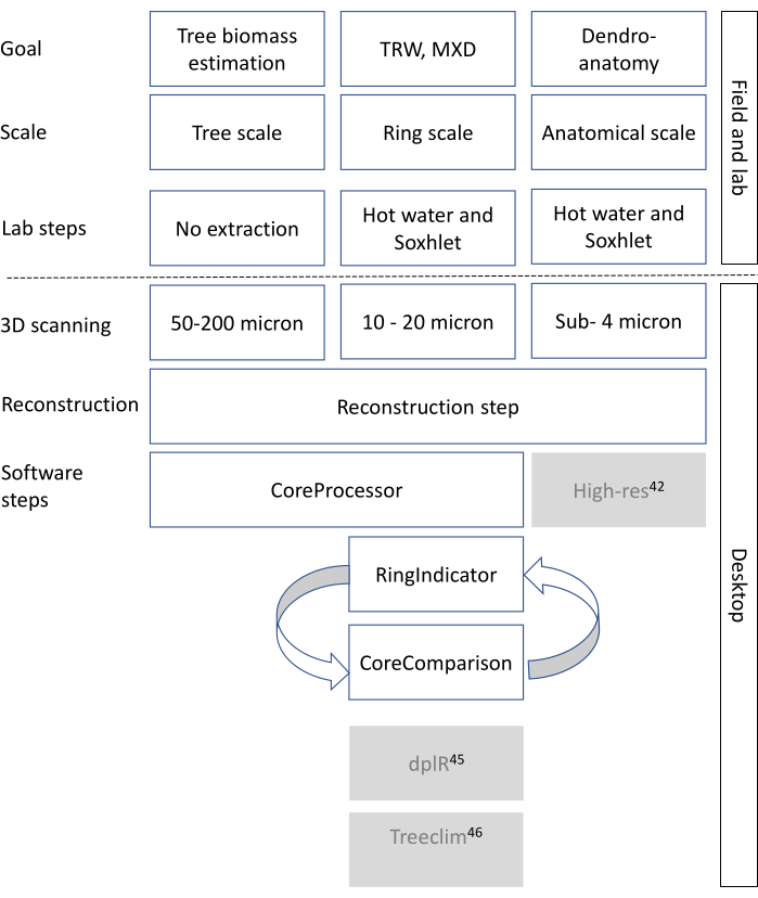
Figure 1: General methodological decision tree for X-ray CT scanning. The rows indicate the steps to take, starting from the research goal all the way to the final data format. White boxes are the steps that are relevant for this toolchain. Greyed-out boxes are steps that can be performed with other software or R packages, such as dplr⁴⁷ and Treeclim⁴⁸ for tree-ring analysis, and ROXAS⁴⁴ as well as ImageJ⁴² or other (commercial) applications for deriving wood anatomical parameters based on the CT images. Please click here to view a larger version of this figure.

X-CT research on wood
Set-up of a scanner: A standard X-ray CT scanner consists of an X-ray tube, an X-ray detector, a rotation stage, and a set of motors to move the rotation stage, and in most cases also the detector, back and forth (Figure 2).

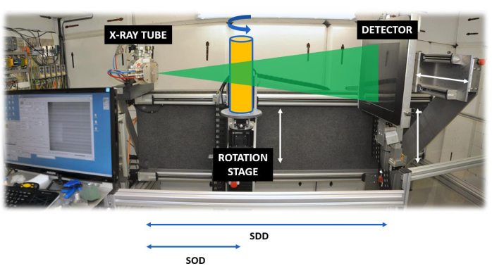
Figure 2. The HECTOR scanning system. The system³⁵, showing the source detector distance (SDD) and the source object distance (SOD). Please click here to view a larger version of this figure.

Most lab-based systems have a cone-beam geometry, which means that the produced X-rays are distributed from the tube's exit window in a cone-beam shape, implying that by changing the distance between the object and the tube (SOD = Source-Object-Distance) and the detector and the tube (SDD = Source-Detector-Distance), the magnification is controlled (see the discussion on resolution). Due to the penetrating power of X-rays, they pass through the object, and the intensity of the attenuation beam is a function of the energy of the X-ray beam, the chemical composition of the object (the atomic number of the elements present) and the density of the material. Given a constant energy spectrum and a constant material composition of wood, the attenuation of the X-ray beam is highly dependent on the density of the material, which explains its use for densitometry. The attenuation (or transmission) can be expressed by the Beer-Lambert law:

with I₀ the incoming X-ray beam exponentially which decays to a transmitted X-ray beam I_d when propagating through the material over a distance d. The linear attenuation coefficient µ depends on a series of interactions with the material of the object. The projections are thus recordings of the transmitted beam.

Practically, the object is mounted on the rotation stage, a proper SOD and SDD are selected, a certain power is selected as well (related to object size, density, and composition) and the object is rotated 360° and during that rotation multiple projections are taken. These projections are then used to reconstruct the interior structure of the object. There are several reconstruction algorithms available, of which the most used ones are still based on the analytical framework developed decades ago, relying on the Radon transformation and the Fourier slice theorem. For more details, the reader is referred to specialized literature³⁶.

Conundrum of resolution, data volume and sample size: Resolution is key in X-ray CT scanning. In systems with inverse geometry, or parallel beam geometry such as synchrotron beamlines, other considerations play a role. This protocol only discusses standard lab-based X-ray CT scanning with cone-beam geometry. Here, the concept of magnification, detector pixel size and spot size are essential. Magnification is defined as the ratio of SDD/SOD. Next, the pixel size of the detector obviously also impacts the resolution: the smaller the pixel size, the higher the resolution, but in most cases the field of view (FoV) is also directly related to pixel size and size of the detector (smaller pixel size, smaller FoV for the same number of pixels). Further, the spot size of the X-ray beam is also important: the larger the spot size, the lower the resolution, which means that less details can be seen.

It is important to address that one could obtain a resolution that is higher than what is possible according to the abovementioned limits, therefore it is better to use the term voxel size (a voxel is a volume pixel) instead of resolution. Moreover, there are other factors at play, such as detector sharpness, which further limit the true resolution at which an object is scanned. Only a true calibration of the system, using established targets, supplies the truthful answer.

In most cases, however, the voxel size at which an object can be scanned is mostly limited by the size of the object. This means that the larger the object, the lower the voxel size will be. If the object does not fit within the FoV of the detector for a certain voxel size, then the voxel size can be reduced, e.g., by limiting the magnification.

Scan time and data volume are important to consider when deciding the desired voxel size. In general, the smaller the voxel size means the higher the detail one wants to see, the smaller the sample or the fewer samples that can be scanned at once, more time is required and larger the data volumes will be collected. Imagine the following theoretical example: one can scan a sample measuring 10 cm x 10 cm x 10 cm at 50 µm at once with a certain X-ray CT system and would like to scan that same volume at 10 µm, the volume that fits within the FoV would only be 2 cm x 2 cm x 2 cm, assuming that this is physically possible. This means that 125 scans are needed (5³ = 5 times higher resolution, scales to the power of 3 due to the volumetric nature of the imaging technique) to cover the entire volume, and that the data volume would increase likewise. Of course, this is only a thought experiment, and one needs to consider much more than only resolution. For more information, the reader is referred to an overview of the scanning possibilities³⁷.

Flexibility of instruments for scanning of wooden objects: In the last decade, many companies have delivered X-ray CT systems with a similar assembly as HECTOR³⁵. An overview of several CT systems, especially assessed for their temporal resolution, is given in³⁸.

In all, the flexibility and user-friendliness of X-ray CT systems has improved considerably. Many systems allow scanning of a diverse range of objects, which is also the case with the systems at UGCT. The protocol below is demonstrated for the HECTOR system, which is suitable for tree-ring analysis. The protocol however is valid for any other available system if resolution and data format allows for it.

These systems allow the scanning of a variety of objects. A few pictures of different wooden objects scanned with the HECTOR system are given in Figure 3. It is this flexibility that comprises the three scales we present in Figure 1, ranging from a coarse resolution to a very fine resolution.

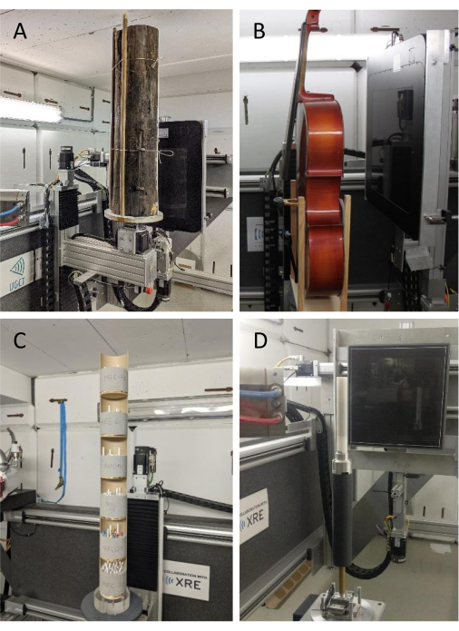
Figure 3. Scanning set-up examples. (A) A log, (B) a cello⁴⁹, (C) sample holders (type 1) with tree cores for batch scanning and (D) sample holder type 2 with increment cores for helical scanning mounted on the rotation stage of HECTOR. Please click here to view a larger version of this figure.

Protocol

1. Core sampling Sample the tree with a Pressler borer. Consult references on how to core a tree manually39. This toolchain is presented for 5.15 mm cores. Put the tree cores unglued into 6 mm paper straws or in any other receptor that does not require glue. Do not glue the tree cores on a wooden support. If the cores were already mounted, unmount them with scalpel/saw or solvent depending on the glue type. Avoid wrapping them in plastic tubes, try …

Representative Results

If the goal is biomass estimation or tree growth increment of many samples, i.e., inter-ring scale (Figure 1), then sample holder 1 (Figure 5) is used to scan samples to obtain density profiles (see step 5.4.3) and estimates of tree growth, e.g., for fast-growing trees with large TRW, which allows for a coarser resolution. Figure 12 shows an example of both pith-to-bark and axial density trends of T. superba, a species from…

Discussion

Critical steps within the protocol
Critical steps within the protocol include proper handling of the increment borer to obtain high-quality increment cores (step 1.1. and see³⁹) to avoid bits and pieces. Next, it is essential that cores be left unmounted (but see²⁶), both for insertion in the sample holder (Figure 5, see²¹) as well as for proper resin extraction⁵⁰ and for possible future ana…

Materials

6 mm paper straws	http://artstraws.com/education/product/artstraws-thick-asst-cols/		Coring
Aluminium core holders
ASTM standard ASTM D 1107 – 96
Cardboard postal tubes	https://www.rajapack.co.uk/envelopes-mailing-bags/postal-tubes/1-5-2mm-brown-cardboard-postal-tubes_PDT05623.html
Column drill
Computer hardware for reconstruction and analysis			X-ray CT scanning
Cooling
Drying oven
Ethanol
Flask for under soxhlet (2000 ml)
Floral foam	https://www.oasisfloral.eu/		Sample holder type 1
Glass beads to fill void volume of Soxhlet to save solvent
Glue
Hot water bath	https://www.memmert.com/products/water-baths/water-bath/#!filters=%7B%7D		Soxhlet extraction
Increment borer	https://haglofsweden.com/project/increment-borers/
Plastic cylinder	Moonen et al. 2022		Sample holder type 2
Plastic cylinders
Reservoir
Tailored soxhlet apparatus
Toluene
Water pump
X-ray CT scanner