JoVE Educación científica
Structural Engineering
Se requiere una suscripción a JoVE para ver este contenido.  Inicie sesión o comience su prueba gratuita.
JoVE Educación científica Structural Engineering
Material Constants
  • 00:07Descripción
  • 01:12Principles of Elasticity Theory
  • 04:40Protocol to Determine Modulus of Elasticity and Poisson’s Ratio
  • 07:41Data Analysis and Results
  • 09:52Applications
  • 10:52Summary

Material Constants

English

Compartir

Descripción

Source: Roberto Leon, Department of Civil and Environmental Engineering, Virginia Tech, Blacksburg, VA

In contrast to the production of cars or toasters, where millions of identical copies are made and extensive prototype testing is possible, each civil engineering structure is unique and very expensive to reproduce (Fig.1). Therefore, civil engineers must extensively rely on analytical modeling to design their structures. These models are simplified abstractions of reality and are used to check that the performance criteria, particularly those related to strength and stiffness, are not violated. In order to accomplish this task, engineers require two components: (a) a set of theories that account for how structures respond to loads, i.e., how forces and deformations are related, and (b) a series of constants that differentiate within those theories how materials (e.g. steel and concrete) differ in their response.

Figure 1
Figure 1: World Trade Center (NYC) transportation hub.

Most engineering design today uses linear elastic principles to calculate forces and deformations in structures. In the theory of elasticity, several material constants are needed to describe the relationship between stress and strain. Stress is defined as the force per unit area while strain is defined as the change in dimension when subjected to a force divided by the original magnitude of that dimension. The two most common of these constants are the modulus of elasticity (E), which relates the stress to the strain, and Poisson's ratio (ν), which is the ratio of lateral to longitudinal strain. This experiment will introduce the typical equipment used in a construction materials laboratory to measure force (or stress) and deformation (or strain), and use them to measure E and ν of a typical aluminum bar.

Principios

Procedimiento

Modulus of Elasticity and Poisson's Ratio It will be assumed herein that students have been trained in the use and safety precautions required to operate a universal testing machine. Obtain a rectangular aluminum bar (12 in. x 1 in. x ¼ in.); an aluminum 6061 T6xxx or stronger is recommended. A hole should be drilled about 1 in. from one beam end to serve as a loading point. Mark a location on the beam about 8.0 in. from the center of …

Resultados

The data should be imported or transcribed into a spreadsheet for easy manipulation and graphing. The data collected is shown in Table 1.

Because the rosette strain gage is not aligned with the principal axes of the beam, the rosette strains need to be input into the equations for ε1,2 (Eq. 9) and ε (Eq. 10) above to compute principal strains, resulting in the data shown in Table 2. The table shows that the angle between the measured stress and the principal stresses is about 0.239 radians or 13.7°. Note that the maximum principal strain is positive, corresponding to a large tensile strain longitudinally; the minimum principal strain is negative, corresponding to a smaller transverse compressive strain. The ratio between the minimum and maximum principal strains corresponds to Poisson's ratio, which is shown on the last column and averages about 0.310.

Load Gage 1 Gage 2 Gage 3 Gage 44
Step (Lbs.) με με με με
1 0.00 1 1 1 0
2 1.10 83 56 -21 -87
3 2.21 163 115 -41 -171
4 3.31 243 171 -62 -254
5 4.42 325 228 -83 -338
6 5.52 400 280 -104 -423
7 6.62 485 338 -122 -501
8 7.73 557 386 -143 -589
9 8.83 634 442 -163 -665
10 9.93 714 502 -184 -741
11 8.83 637 445 -162 -664
12 7.73 561 391 -142 -584
13 6.62 483 335 -123 -506
14 5.52 406 281 -102 -423
15 4.42 323 227 -83 -339
16 3.31 245 171 -62 -256
17 2.21 164 115 -41 -170
18 1.10 83 56 -21 -87
19 0.00 1 0 1 2

Table 1: Strains in aluminum bar.

Gage Factor 1 2 3 Maximum Principal Strain Minimum. Principal Strain Angle Poisson's Ratio
Load step με με με (Eq. 9) (Eq. 9) (Eq. 10) (Eq. 7)
1 1 1 1 1 1 0 0
2 83 56 -21 89 -26 -0.223 0.297
3 163 115 -41 176 -55 -0.243 0.311
4 243 171 -62 263 -82 -0.242 0.312
5 325 228 -83 351 -109 -0.240 0.311
6 400 280 -104 432 -136 -0.240 0.314
7 485 338 -122 523 -160 -0.237 0.307
8 557 386 -143 600 -186 -0.236 0.310
9 634 442 -163 684 -213 -0.238 0.312
10 714 502 -184 773 -242 -0.242 0.314
11 637 445 -162 688 -213 -0.239 0.309
12 561 391 -142 605 -186 -0.237 0.308
13 483 335 -123 520 -161 -0.236 0.309
14 406 281 -102 437 -133 -0.234 0.303
15 323 227 -83 349 -109 -0.241 0.313
16 245 171 -62 264 -81 -0.238 0.308
17 164 115 -41 177 -54 -0.239 0.302
18 83 56 -21 89 -26 -0.223 0.297
19 1 0 1 2 0 0.000 0.000
Average -0.239 0.310

Table 2: Principal strains and angle of inclination.

The maximum and minimum principal strains from Table 2 are plotted in Fig. 5 which shows very linear trends (R2 = 0.999) for Poisson's ratio. The value obtained for Poisson's ratio (0.31), which corresponds to the slope of the line, is very close to the 0.30 given in most references for aluminium and other metals.

Figure 5
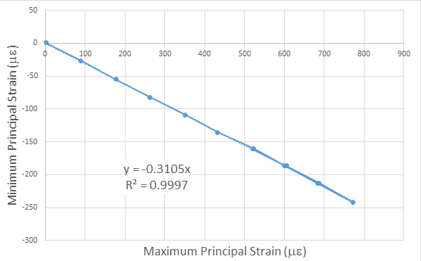
Figure 5: Principal strain data showing the slope of the line between maximum and minimum principal strain, which corresponds to Poisson's ratio.

A good physical interpretation of the rosette strain gage data can be gained from plotting the principal strains on a Mohr circle (Fig. 6). Note that the three measurements, shown here for the case of the maximum load of 7.4 lbs., correspond to three points in the circle at 90º to one another, starting at an angle of about 27.4º (or) counterclockwise from the x-axis.

Figure 6
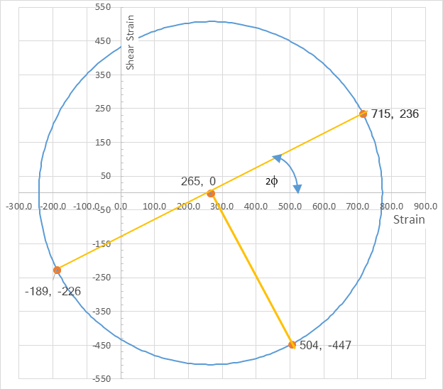
Figure 6: Physical significance of strain rosette readings shown on Mohr's circle for strain.

Table 3 shows the loads, the results for the principal tensile strain from the single gage on the underside of the beam (Gage 4, which is in compression), the ratio between the bottom and top maximum principal stresses, the stress from Eq. (11), and Young's modulus (E) as the ratio of the stress from Eq. (11) divided by the strain from Eq. (9). In Table 3, a Young's modulus is calculated as 10147 ksi by taking the average of the moduli calculated for the 15 intermediate loading steps.

Load Max. Principal. Strain Max Principal Stress Min Principal Stress Bending Stress Young' Modulus
Load step Lbs. με ksi ksi psi ksi
1 0.00 1 10 9 0 0
2 1.10 89 886 0 882 9945
3 2.21 176 1765 0 1763 9991
4 3.31 263 2630 0 2645 10058
5 4.42 351 3513 0 3526 10038
6 5.52 432 4324 0 4408 10195
7 6.62 523 5230 0 5290 10113
8 7.73 600 6001 0 6171 10283
9 8.83 684 6843 0 7053 10307
10 9.93 773 7726 0 7935 10269
11 8.83 688 6877 0 7053 10256
12 7.73 605 6051 0 6171 10198
13 6.62 520 5204 0 5290 10165
14 5.52 437 4368 0 4408 10091
15 4.42 349 3494 0 3526 10092
16 3.31 264 2644 0 2645 10004
17 2.21 177 1770 0 1763 9960
18 1.10 89 886 0 882 9945
19 0.00 2 19 0 0 0
Average 10147

Table 3: Calculation of modulus of elasticity (E).

The data for E is also plotted in Fig. 7, which indicates an excellent linear relationship (high R2) between stress and strain and a slope of about 10,147 ksi. The difference between the modulus from Table 3 and that from Fig. 6 arises because the calculations for the slope in Fig. 6 require that the intercept go through zero. The magnitudes compare very favourably (error less than 1.5%) with published values of E for 6061T6 aluminium, which is usually given as 10,000 ksi.

Figure 7
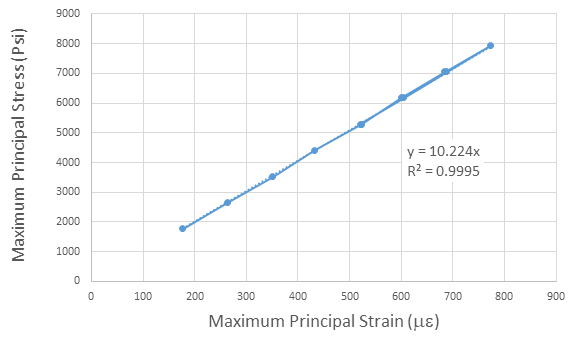
Figure 7: Slope of line of maximum stress vs. maximum strain is Young's modulus.

Finally, by recasting Eqs. (5) and (6) into:
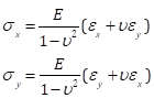
Equation 12 (Eq. 12)

we can calculate the principal stresses using Mohr's circle. For the case of the step corresponding to 6.61 lbs. of load, the principal strains of (634, -189) lead to principal stresses of (7.34, 0.00) ksi (Fig. 8). Although the calculations here are done using the expressions for plane stress, the results correctly indicate that along the principal axis the stress in the perpendicular direction is zero (or very close to it), corresponding to the case of uniaxial loading. The stress values at an angle of 2Φ = 0.40 radians are (6.50, 2.82) ksi.

Figure 8
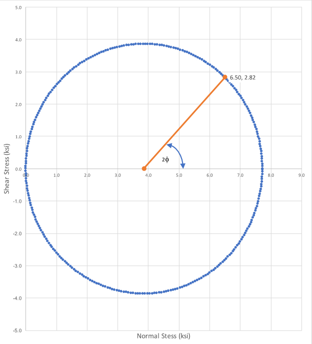
Figure 8: Mohr's circle for plane stress for the case of a 7.34 lbs load.

Applications and Summary

In this experiment, two fundamental material constants were measured: the modulus of elasticity (E) and Poisson's ratio (v). This experiment demonstrates how to measure these constants in a laboratory setting using a rosette strain gage. The values obtained experimentally match well with the published values of 10,000 ksi and 0.3, respectively. These values are key in applying the theory of elasticity for engineering design, and this experimental technique described herein are typical of those used for obtaining materials constants. To obtain these values, great care must be taken both in utilizing high resolution instrumentation and traceable calibration procedures. In particular, the use of strain gage-based devices and 16 to 24-bit digital data acquisition systems are integral to the success and quality of such experiments.

Today, there are other methods of determining Young's modulus of a material, including wave propagation methods (ultrasonic echo-pulse method) and nanoindentation. One benefit of utilizing wave propagation is that it is one of the non-destructive methods of measuring Young's modulus, whereas nanoindentation and use of a rosette strain gage are more invasive methods.

The design of any engineering product, from a toaster to a skyscraper, requires the use of effective analytical models to improve and optimize the design. The theory of elasticity is the foundation of most models used in civil engineering design, and is based upon the establishment of several constants.

Analytical models are required when only a single (or very few) replicates will be built. As the cost and performance of the structure depend on the result of those analyses, and those analyses, in turn, depend on having robust values for the material properties, tests such as the ones described here must be run to ensure quality control and quality assurance in the construction process. For example:

  • In choosing a façade for a building, the architect must be careful to design a waterproof envelope. The water tightness of a brick building façade may depend on maintaining the mortar between the bricks uncracked, among other factors. If the mortar cracks, water will penetrate and cause corrosion and humidity problems which will be very expensive to fix. In order to determine how much force the mortar can resist before it cracks, we need both a theory and its associated constants. The architect and structural engineer must work together to determine what loads the façade will see (self-weight, wind, driving rain, etc.) and how each design option will perform under those conditions. Only then can a mortar with the appropriate characteristics should be chosen.
  • In constructing a tall building, such as the Burj Dubai, the construction company needs to pay close attention to keeping the floors level. As the construction progresses, if the sizes of the columns and walls are different, some of these elements may shorten (strain) more than others as the construction progresses and more weight (stress) is added. To obtain flat floors at the end of construction, the construction company will need to make adjustments to the height of the columns and walls in the lower floors – the lower floors may not be level during the initial phases of construction but should be flat at the end. To calculate how to properly make these adjustments, the construction company will hire a structural engineer to provide data on differential column and wall heights. The engineer will need to use material constants to carry out these computations.
  • In the design of a soda can, a manufacturer must minimize the thickness of the aluminum wall, as aluminum is a very expensive material. To optimize the shape and dimensions of the cans, the manufacturer needs to determine what loading conditions are important; transportation and storage conditions may be more demanding than the consumer drinking from it. Many of these conditions will be hard and expensive to replicate within an experimental testing program; the manufacturer may choose to do a lot of analysis to optimize the can dimensions before moving to the prototype phase. This procedure is what Boeing followed in developing the Dreamliner (Boeing 787). To do these studies, material properties must be known and the appropriate theory selected.

Transcripción

Most engineering design today uses the theory of elasticity and several material constants to estimate the performance criteria of a structure.

In contrast to the production of cars, for example, where millions of identical copies are made, an extensive prototype testing is possible. Each civil engineering structure is unique, and its design vastly relies on an analytical modeling and different material constants.

The two most common material constants used in civil engineering design are the Modulus of Elasticity, which relates stress to strain, and Poisson’s Ratio, which is the ratio of lateral to longitudinal strains.

In this video, we will measure stress and strain with equipment typically found in a construction materials laboratory, and use these quantities to determine the material constants of an aluminum bar.

The most common model used for analysis is linear elasticity, or Hooke’s Law, which postulates that the applied force is directly proportional to deformation.

In engineering, stress is defined as the force per unit area, while strain is defined as the change in dimension when subjected to a force, divided by the original magnitude of that dimension. According to Hooke’s Law, stress is proportional with strain, and the constant of proportionality is the constant of elasticity. If we can measure the force, the strain, and the original area, we can find E. This is the particular case of a unit directional load.

Let’s look now at the general case where a piece of structure is subjected to 3D loads. Considering an X, Y, Z coordinate system, at any given point the solid body is subjected to three normal components and three sheer components of stress. Breaking the equations of equilibrium for forces and moments along all axes results in a series of equations for the normal strain and the sheer strain.

Six equations of this type, three for normal strains and three for sheer strains, are needed to establish the global deformations. These equations contain three constants, the Modulus of Elasticity (E), Poisson’s Ratio (μ), and the Sheer Modulus (G). The Sheer Modulus is defined as the change in angular deformation given the sheer stress or surface traction. Poisson’s Ratio is defined as the ratio of transversal to longitudinal strain. Since G can be expressed using E and μ, only two of the three constants need to be measured in order to define all three.

For the state of stress, represented in the X, Y, Z coordinate system, there is an equivalent representation on a new coordinate system of principal axes one, two, and three, where there are no sheer stresses. The normal stresses in this particular system are called Principal Normal Stresses. Among these, there is a minimum and respectively maximum principal stress acting on any plane. The state of stress and strain on a surface is determined if at least three independent strain measurements are made.

In the laboratory, a rosette strain gauge composed of three strain gauges aligned at 45 degrees to one another, is used to measure strain in three different directions. From here, the complete state of stress on a surface can be defined using Mohr’s circle, to calculate maximum and minimum principal strains and the angle between the measured strains and the principal strains.

In this experiment, we will use a simple cantilever beam instrumented with strain gauges to illustrate the concepts of principal strains and stresses and measure the Young’s Modulus and the Poisson’s Ratio.

Obtain a regular aluminum bar, of dimensions 12 inches by 1 inch by 1/4 inch. An aluminum 6061-T6 or stronger is recommended.

Drill a hole at one end of the beam to serve as a loading point, and mark a location on the beam, about eight inches from the center of the hole, where the strain gauges will be installed. Measure area of the bar carefully, using calipers. Perform three replicates in three different locations, to obtain a good average of the dimensions. From these measurements, calculate the moment of inertia of the bar.

Next, obtain a rosette strain gauge with a sensing grid of approximately 1/4 inch long by 1/8 inch wide on each gauge. Note the calibration factor or gauge factor. Mark the location where the strain gauge will be installed. Then, degrease this area, obtain a very smooth surface by sanding with progressively finer grades of sandpaper, clean the surface with a neutralizer. Mix the epoxy components and install the strain gauges. Installation and glue curing procedures should follow manufacturer specifications.

Make sure to test the resistance of the gauges using an ohm meter and their current leakage to the specimen bar before proceeding. A micro-measurements 1300 strain gauge tester will be used herein for this purpose. Repeat these operations to install a single strain gauge longitudinally on the surface and directly below the strain gauge rosette.

Insert the specimen into a secure vice, that ensures the aluminum beam will behave as a cantilever beam. Now, connect the strain gauges to a recording device. Make sure that the wiring is correct as per the strain indicator instructions, and that you know which channel corresponds to each strain gauge.

Then, enter the appropriate gauge factors for each gauge in the indicator. If possible, calibrate the strain gauge outputs and the strains in the indicator. Make sure to record initial load and strains. Now, slowly apply seven increments of 0.5 kilograms of load at the beam tip. Pause at every step and allow measurements to stabilize before recording readings. Next, slowly apply eight decrements of 0.5 kilograms. Make sure to pause at every step and allow measurements to stabilize before recording readings.

Raw data shown in the table consists of the load step number, applied loads, the strain from the top rosette strain gauge, and the strain from the single bottom strain gauge. The initial and final load steps will not be used in the calculations, as the readings are small and will not produce accurate results.

Next, using the strain values from the top rosette strain gauge, compute the principal strains, the angle of inclination, and the Poisson’s ratio as the ratio of the maximum to minimum principal strain. Plotting the maximum and minimal principal strains corresponds to plotting the longitudinal and transfer strains; and thus, the slope of this line corresponds to Poisson’s ratio. The value obtained is very close to the generally accepted value of 0.3, and the R squared measure indicates very good linearity.

A good physical interpretation of the rosette strain gauge data can be gained from plotting the principal strains on a Mohr’s circle. Note that the three measurements shown here for the case of the maximum load of 9.93 pounds corresponds to three points in the circles at 90 degrees to one another, starting at an angle of about 27.4 degrees, counter-clockwise from the X axis.

Next, from the load values we calculate the bending stresses. The Young’s Modulus is given by the ratio of the stress of the maximum principal strain, which we had calculated in Table 2. Now, plot the stress versus strain, and compute the slope of this line, which corresponds to Young’s Modulus. The value obtained is very close to the theoretical value of 10,000 KSI. Finally, draw the Mohr’s circle for plane stress.

Material constants are used together with theoretical models to improve and optimize the design of many engineering products, from consumer goods to aircrafts and skyscrapers.

For waterproofing the facade of a brick building, the engineer must determine, among other factors, how much force the mortar between bricks can resist before it cracks. Different analytical models and material constants are employed in order to decide what type of mortar should be chosen for construction, based on the load that the facade will likely see.

In the design of a soda can, a manufacturer must minimize the thickness of the aluminum wall in order to decrease the costs. Before moving to the prototype phase, theoretical studies taking into account the material properties may be performed in order to optimize the can shape and dimensions.

You’ve just watched JoVE’s Introduction to Material Constants. You should now understand the basics of the theory of elasticity. You should also know how to measure the Modulus of Elasticity and the Poisson’s ratio, two fundamental material constants widely used for practical engineering applications.

Thanks for watching!

Tags

Cite This
JoVE Science Education Database. JoVE Science Education. Material Constants. JoVE, Cambridge, MA, (2023).