Se requiere una suscripción a JoVE para ver este contenido.  Inicie sesión o comience su prueba gratuita.
Growth Curves: Generating Growth Curves Using Colony Forming Units and Optical Density Measurements
  • 00:01Concepts
  • 03:44Set-Up
  • 08:52Data Analysis and Results

Curve di crescita: generazione di curve di crescita utilizzando le unità formanti colonia e la misurazione della densità ottica

English

Compartir

Descripción

Fonte: Andrew J. Van Alst1, Rhiannon M. LeVeque1, Natalia Martin1e Victor J. DiRita1
1 Dipartimento di Microbiologia e Genetica Molecolare, Michigan State University, East Lansing, Michigan, Stati Uniti d’America

Le curve di crescita forniscono preziose informazioni sulla cinetica di crescita batterica e sulla fisiologia cellulare. Ci permettono di determinare come i batteri rispondono in condizioni di crescita variabili e di definire parametri di crescita ottimali per un determinato batterio. Una curva di crescita archetipica progredisce attraverso quattro fasi di crescita: ritardo, esponenziale, stazionaria e morte (1).

Figure 1
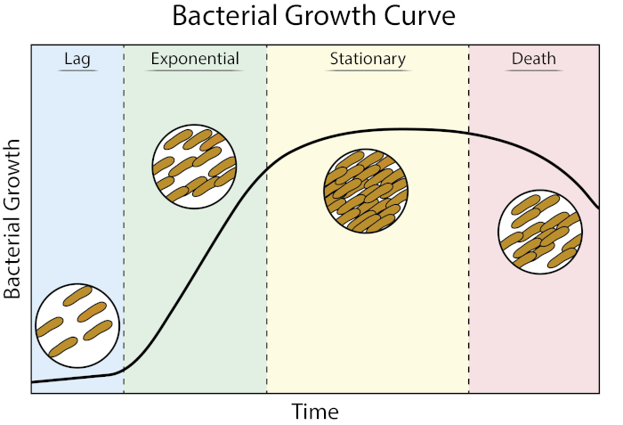
Figura 1: Curva di crescita batterica. I batteri cresciuti in coltura batch progrediscono attraverso quattro fasi di crescita: ritardo, esponenziale, stazionario e morte. La fase di ritardo è il periodo di tempo necessario ai batteri per raggiungere uno stato fisiologico in grado di una rapida crescita e divisione cellulare. La fase esponenziale è lo stadio di crescita e divisione cellulare più veloce durante il quale la replicazione del DNA, la trascrizione dell’RNA e la produzione di proteine avvengono tutte a un ritmo costante e rapido. La fase stazionaria è caratterizzata da un rallentamento e plateau della crescita batterica dovuto alla limitazione dei nutrienti e/o all’accumulo intermedio tossico. La fase di morte è la fase durante la quale si verifica la lisi cellulare a causa di una grave limitazione dei nutrienti.

La fase di ritardo è il periodo di tempo necessario ai batteri per raggiungere uno stato fisiologico in grado di una rapida crescita e divisione cellulare. Questo ritardo si verifica perché ci vuole tempo perché i batteri si adattino al loro nuovo ambiente. Una volta che i componenti cellulari necessari sono generati in fase di ritardo, i batteri entrano nella fase esponenziale di crescita in cui la replicazione del DNA, la trascrizione dell’RNA e la produzione di proteine avvengono tutte a un ritmo costante e rapido (2). Il tasso di rapida crescita e divisione cellulare durante la fase esponenziale è calcolato come il tempo di generazione, o tempo di raddoppio, ed è il tasso più veloce al quale i batteri possono replicarsi nelle condizioni date (1). Il tempo di raddoppio può essere utilizzato per confrontare diverse condizioni di crescita per determinare quale è più favorevole per la crescita batterica. La fase di crescita esponenziale è la condizione di crescita più riproducibile in quanto la fisiologia delle cellule batteriche è coerente in tutta la popolazione (3). La fase stazionaria segue la fase esponenziale in cui la crescita cellulare si stabilizze. La fase stazionaria è causata dall’esaurimento dei nutrienti e / o dall’accumulo di intermedi tossici. Le cellule batteriche continuano a sopravvivere in questa fase, anche se il tasso di replicazione e divisione cellulare è drasticamente ridotto. La fase finale è la morte, dove un grave esaurimento dei nutrienti porta alla lisi delle cellule. Le caratteristiche della curva di crescita che forniscono la maggior parte delle informazioni includono la durata della fase di ritardo, il tempo di raddoppio e la densità massima della cella raggiunta.

La quantificazione dei batteri in coltura batch può essere determinata utilizzando sia le unità formanti colonie che le misurazioni ottiche della densità. L’enumerazione per unità formanti colonie (CFU) fornisce una misurazione diretta della conta delle cellule batteriche. L’unità di misura standard per i CFU è il numero di batteri coltivabili presenti per 1 mL di coltura (CFU/mL) determinato mediante tecniche di diluizione seriale e placcatura diffusa. Per ogni punto temporale, viene eseguita una serie di diluizione 1:10 della coltura batch e 100 μl di ciascuna diluizione vengono distribuiti placcati utilizzando uno spandiconci cella.

Figure 2
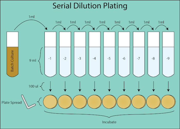
Figura 2. Schema di placcatura a diluizione seriale. Flusso generale per la placcatura di diluizione da coltura batch. La coltura del lotto viene diluita in serie 1:10 trasferendo 1 mL della diluizione precedente nel tubo successivo contenente 9 ml di PBS. Da ogni tubo di diluizione, 100 μl vengono distribuiti placcati utilizzando uno spandipiatti che è una diluizione aggiuntiva di 1:10 in quanto è 1/10 del volume di 1 mL di volume nel calcolo di CFU / mL. Le piastre vengono incubate ed enumerate una volta che le colonie clonali crescono sulle piastre.

Le placche vengono quindi incubate durante la notte e le colonie clonali enumerate. La piastra di diluizione che ha coltivato 30-300 colonie viene utilizzata per calcolare il CFU/ mL per il punto temporale dato (4, 5). La variazione stocastica nel conteggio delle colonie inferiore a 30 è soggetta a un errore maggiore nel calcolo dei CFU/mL e il conteggio delle colonie superiori a 300 può essere sottovalutato a causa dell’affollamento e della sovrapposizione delle colonie. Utilizzando il fattore di diluizione per la piastra data, è possibile calcolare il CFU della coltura batch per ciascun punto temporale.

La densità ottica fornisce un’approssimazione istantanea della conta cellulare batterica misurata utilizzando uno spettrofotometro. La densità ottica è una misura dell’assorbanza delle particelle di luce che passano attraverso 1 cm di coltura e rilevate da un sensore di fotodiodi (6). La densità ottica di una coltura viene misurata in relazione a un mezzo vuoto e aumenta all’aumentare della densità batterica. Per le cellule batteriche, una lunghezza d’onda di 600 nm (OD600) viene in genere utilizzata quando si misura la densità ottica (4). Generando una curva standard relativa alle unità formanti colonie e alla densità ottica, la misurazione della densità ottica può essere utilizzata per approssimare facilmente il conteggio delle cellule batteriche di una coltura batch. Tuttavia, questa relazione inizia a deteriorarsi già a 0,3 OD600 quando le cellule iniziano a cambiare forma e ad accumulare prodotti extracellulari nel mezzo, influenzando la lettura della densità ottica in relazione ai CFU (7). Questo errore diventa più pronunciato durante le fasi stazionarie e di morte.

Qui, L’Escherichia coli viene coltivata in brodo Luria-Bertani (LB) a 37°C nel corso di 30 ore (7). Sono state generate sia curve di crescita CFU/mL che curve di crescita della densità ottica, nonché la curva standard che correla la densità ottica con cFU.

Figure 3
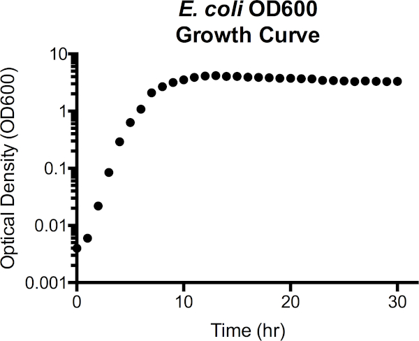
Figura 3. Densità ottica di Escherichia coli alla curva di crescita della lunghezza d’onda di 600 nm (OD600). I valori di densità ottica sono stati prelevati direttamente dallo spettrofotometro dopo l’oscuramento con supporti LB sterili. I valori di OD600 superiori a 1,0 sono stati diluiti 1:10 combinando la coltura di 100 μl con LB fresco di 900 μl, nuovamente misurato, e quindi moltiplicato per 10 per ottenere il valore OD600. Questo passo viene fatto quando la precisione nella misurazione dello spettrofotometro viene ridotta ad alta densità di cellule. Dalla curva, la fase di ritardo si estende a circa 1 ora di crescita, passa alla fase esponenziale da 2h a 7h, quindi inizia a stabilizzarsi, entrando in fase stazionaria. La fase di morte non è una transizione netta, tuttavia, poiché la densità ottica inizia gradualmente a diminuire dopo 15 ore.

Figure 4
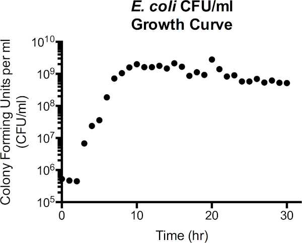
Figura 4. Unità formante colonia di Escherichia coli per millilitro (CFU/mL) curva di crescita. I valori di CFU/mL per ogni timepoint sono stati calcolati dalla piastra di diluizione che conteneva 30-300 colonie. Dalla curva, la fase di ritardo si estende fino a circa 2 ore di crescita, passa alla fase esponenziale da 2h a 7h, quindi inizia a stabilizzarsi, entrando in fase stazionaria. La fase di morte non è una transizione netta, tuttavia, poiché CFU / mL inizia gradualmente a diminuire dopo 15 ore da un picco di 2 x 10⁹ a circa 5 x 10⁸ a 30 ore.

Figure 5
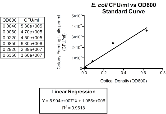
Figura 5. Curva di standardizzazione per CFU/mL rispetto a OD600. Una regressione lineare può essere utilizzata per correlare queste unità in modo che la densità ottica possa essere utilizzata per approssimare la densità cellulare batterica. La densità ottica può essere utilizzata per fornire un’approssimazione istantanea del CFU/mL della coltura batch. Qui, vengono tracciati solo i primi sei punti temporali poiché la relazione tra OD600 e CFU / mL è meno accurata oltre 1,0 OD600 poiché la forma cellulare e i prodotti extracellulari iniziano ad accumularsi quando i batteri entrano in fase stazionaria, che si verifica poco dopo aver raggiunto 1,0 OD600. I cambiamenti nella forma cellulare e nei prodotti extracellulari nei media influenzano la lettura della densità ottica e quindi anche la relazione tra densità ottica e numero di batteri nella coltura è influenzata.

Anche il tempo di raddoppio è stato determinato in 15 minuti e 19 secondi. Da questi dati, la capacità di crescita in LB per E. coli può essere visualizzata ed essere utilizzata per il confronto tra diversi mezzi o batteri.

Procedimiento

1. Configurazione Materiali di laboratorio richiesti: mezzi liquidi, mezzi di agar solidificati, palloni Erlenmeyer, provette da 15 ml, soluzione salina tamponata con fosfato (PBS), diffusore di cellule batteriche, etanolo al 70% e uno spettrofotometro. Tutte le soluzioni e i bicchieri devono essere sterilizzati prima dell’uso. Preparare la postazione di lavoro sterilizzando con etanolo al 70%. Lavora vicino a un bruciatore Bunsen per prevenire la contaminazione dei supporti. <l…

Resultados

Plots of colony forming units and optical density are two ways to visualize growth kinetics. By determining the relationship between CFU/mL and OD600, the optical density plot also provides an estimate of CFU/mL over time. Conditions that result in the shortest doubling time are considered optimal for growth of the given bacteria.

Applications and Summary

Growth curves are valuable for understanding the growth kinetics and physiology of bacteria. They allow us to determine how bacteria respond in variable growth conditions as well as define the optimal growth parameters for a given bacterium. Colony forming unit and optical density plots both contain valuable information depicting the duration of lag phase, maximum cell density reached, and allowing for the calculation of bacterial doubling time. Growth curves also allow for comparison between different bacteria under the same growth conditions. Additionally, optical density provides a means of standardizing initial inoculums, enhancing consistency in other experiments.

Determining which approach to use when designing a growth curve experiment requires consideration. As the preferred method for generating growth curves, colony forming unit plots more accurately reflect the viable cell counts in batch culture. Colony forming unit plots also allow for measuring bacterial growth in conditions that would otherwise interfere with an optical density measurement. However, it is a more time consuming process, requiring extensive use of reagents, and must be performed manually. Optical density plots are less accurate and provide only an estimate of the colony forming units, requiring a standard curve to be generated for each unique bacteria. Optical density is primarily used for its convenience as it is far less time consuming and does not require many reagents to perform. What is most attractive to optical density, is that spectrophotometric incubators can automatically generate growth curves, vastly increasing the number of culture conditions that can be tested at once and eliminating the need to constantly attend the culture.

Referencias

  1. R. E. Buchanan. 1918. Life Phases in a Bacterial Culture. J Infect Dis 23:109-125.
  2. CAMPBELL A. 1957. Synchronization of cell division. Bacteriol Rev 21:263-72.
  3. Wang P, Robert L, Pelletier J, Dang WL, Taddei F, Wright A, Jun S. 2010. Robust growth of Escherichia coli. Curr Biol 20:1099-103.
  4. Goldman E, Green LH. 2015. Practical Handbook of Microbiology, Third Edition. CRC Press.
  5. Ben-David A, Davidson CE. 2014. Estimation method for serial dilution experiments. J Microbiol Methods 107:214-221.
  6. Koch AL. 1968. Theory of the angular dependence of light scattered by bacteria and similar-sized biological objects. J Theor Biol 18:133-156.
  7. Sezonov G, Joseleau-Petit D, D'Ari R. 2007. Escherichia coli physiology in Luria-Bertani broth. J Bacteriol 189:8746-9.

Transcripción

Bacteria reproduce through a process called cell division, which results in two identical daughter cells. If the growth conditions are favorable, bacterial populations will grow exponentially.

Bacterial growth curves plot the amount of bacteria in a culture as a function of time. A typical growth curve progresses through four stages: lag phase, exponential phase, stationary phase, and death phase. The lag phase is the time it takes for bacteria to reach a state where they can grow and divide quickly. After this, the bacteria transition to the exponential phase, characterized by rapid cell growth and division. The rate of exponential growth of the bacterial culture during this phase can be expressed as the doubling time, the fastest rate at which bacteria can reproduce under specific conditions. The stationary phase comes next, where bacterial cell growth plateaus and the growth and death rates even out due to environmental nutrient depletion. Finally, the bacteria enter the death phase. This is where bacterial growth declines sharply and severe nutrient depletion leads to the lysing of cells.

Two techniques can be used to quantify the amount of bacteria present in a culture and plot a growth curve. The first of these is via colony forming units, or CFUs. To obtain CFUs a one to ten series of nine dilutions is performed at regular time points. The first of these dilutions, negative one in this example, contains 9mL of PBS and 1mL of the bacterial culture. Resulting in a 1:10 dilution factor. Then, 1mL of this solution is transferred to the next tube, negative two, resulting in a 1:100 dilution factor. This process continues through the last tube, negative nine, resulting in a final dilution factor of 1:1 billion. After this, 100 microliters of each dilution is plated. The plates are then incubated and the clonal colonies are counted. The dilution plate for a given time point that grows between 30 and 300 colonies is used to calculate the CFUs per milliliter for that time point.

The second common method of measuring bacterial concentration is the optical density. The optical density of a culture can be measured instantly, in relation a media blank, with a spectrophotometer. Typically a wave length of 600 nanometers, also referred to as OD600, is used for these measurements, which increase as cell density increases. While optical density is less precise than CFUs, it is convenient because it can be obtained instantaneously and requires relatively few reagents. Both techniques can be used together to create a standard curve that more accurately approximates the bacterial cell count of a culture. In this video, you will learn how to obtain CFUs and OD600 measurements from timed serial dilutions of E. coli. Then, two growth curves using the CFU and OD600 measurements, respectively, will be plotted before being related by a standard curve.

When working with bacteria, it is important to use the appropriate personal protective equipment such as a lab coat and gloves and to observe proper aseptic technique.

After this, sterilize the work station with 70% ethanol. First, prepare the LB broth and LB solid agar media in separate autoclaveable bottles. After partially closing the caps of the bottles, sterilize the media in an autoclave set to 121 degrees Celsius for 35 minutes. Next, allow the agar media to cool in a water bath set to 50 degrees Celsius for 30 minutes. Once cooled, pour 20 to 25 mL into each Petri dish. After this, allow the plates to set for 24 hours at room temperature.

To prepare the single colony isolates that will later be used to produce a liquid bacterial culture, use previously frozen stock and proper streak plating technique to streak E. coli for isolation on LB agar. Incubate the dish at 37 degree Celsius overnight. After this, cool a flame sterilized inoculation loop on the agar before selecting a single colony from the streaked plate. Inoculate 4 mL of liquid media in a 15 mL test tube. Then, grow the E. coli at 37 degrees Celsius overnight with shaking at 210 rpm.

To set up the 1:1000 volume of bacterial culture that will be used in the growth curve, first obtain an autoclaved 500 mL Erlenmeyer flask. Then, use a 50 mL serological pipette to transfer 100 mL of sterile media to the flask. Next, label nine 15 ml test tubes consecutively as one through nine. These numbers correspond to the dilution factor that will be used to calculate the colony forming unit, or CFU. Then, add 9 mL of 1X PBS to each tube. After this, label the prepared agar plates with the corresponding time points and dilution factors that will be grown. In this example with E. coli, after the starting time point, time points are taken once every hour. Using the previously prepared overnight liquid E. coli culture, inoculate the media in the autoclave 500 mL Erlenmeyer flask with 1:1000 volume of culture. Swirl the media to evenly distribute the bacteria.

After blanking a spectrophotometer, clean the cuvette with a lint-free wipe. Next, dispense 1 mL of the culture into the cuvette and place it into the spectrophotometer to obtain the optical density of the culture at time point zero. Then, grow the E. coli at 37 degrees Celsius with shaking at 210 rpm. At each time point after time point zero, withdraw another 1 mL of bacterial culture from the flask and repeat the optical density measurement. If the optical density reading is greater than 1.0, dilute 100 microliters of bacterial culture with 900 microliters of fresh media and then measure the optical density once more. This value can be multiplied by 10 for the OD 600 measurement.

To obtain the colony forming unit measurement for each time point, withdraw an additional 1 mL of bacterial culture from the flask at each time point. Dispense the bacterial culture into the negative one test tube and vortex to mix. Then, perform the dilution series by first transferring 1 mL from the negative one tube into the negative two tube and vortex to mix. Transfer 1 mL from the negative two tube into the negative three tube and vortex to mix. Continue this serial transfer down all the dilution tubes to the negative nine tube. Dispense 100 microliters of cell suspension onto the correspondingly labeled plate for each dilution. For every dilution, sterilize a cell spreader in ethanol, pass it through a Bunsen burner flame, and cool it by touching the surface of the agar away from the inoculate. Then, use the cell spreader to spread the cell suspension until the surface of the agar plate becomes dry. Incubate the plates upside down at 37 degrees Celsius. Once visible colonies arise, count the number of bacterial colonies on each plate. Record these values and their associated dilution factors for each plate at each time point.

To create an OD 600 growth curve, after ensuring all the data points are entered correctly into a table, select all of the time points and their corresponding data. To generate a colony forming unit growth curve plot, choose the dilution plate where the colony counts fell within the range 30 to 300 bacteria for each time point. Multiply the colony count number by the dilution factor, and then by ten. This is because the 100 microliters spread is considered an additional 1:10 dilution when calculating colony forming units per milliliter. After this, plot the colony forming units versus time on a semi-log scale.

These plots produced with OD 600 and CFU measurements, respectively, can provide valuable information on E. coli growth kinetics. The optical density and colony forming units can be related, so that CFUs per milliliter can be estimated from OD 600 measurements, saving time and materials in future experiments.

To do this, plot the colony forming units against the optical density on a linear scale for OD 600 readings less than or equal to 1. 0. After this, generate a linear regression trend line in Y = MX + B format, where M is the slope and B is the y-intercept. Right click on the data points and select add trend line and linear. Then, check the box to display the equation on the chart and display the R squared value on the chart. The R squared value is the statistical measurement of how closely the data matched the fitted regression line. In this example, the first 6 time points are plotted with OD 600 on the x axis and CFUs per milliliter on the y axis. In future experiments with the same growth conditions, these slope and y-intercept values can be plugged into this equation to estimate CFUs from OD 600 readings. Next, look at the colony forming unit growth curve plot. During the exponential phase, identify two time points with the steepest slope between them. To calculate the doubling time, first calculate the change in time between the selected time points. Then, calculate the change in generations using the equation shown here. Here, lower case b is the number of bacteria at time point three and upper case B is the number of bacteria at time point two. Finally, divide the change in time by the change in generations. In this example, the doubling time is 0. 26 hours or 15 minutes and 19 seconds. Comparing doubling times across different experimental treatment allows us to identify the best growth conditions for a certain bacterial species. Therefore, the treatment with the lowest doubling time will be most optimal of the conditions tested.

Tags

Cite This
JoVE Science Education Database. JoVE Science Education. Growth Curves: Generating Growth Curves Using Colony Forming Units and Optical Density Measurements. JoVE, Cambridge, MA, (2023).