Quenching is a heat treatment commonly used to modify material properties such as hardness and ductility. During quenching and the complementary process of annealing, a material is heated and subsequently cooled. For quenching, the material is cooled very quickly in contrast to annealing where it is cooled gradually in a controlled fashion. The rate of heat transfer is determined by many factors including the thermal conductivity of an object and surrounding fluid, geometry and temperature distribution. Understanding the interplay between these factors is important for building the link between a particular heat treatment and the resulting change in material properties. This video will focus on quenching and show how to perform a simple analysis of the heat transfer during this process.
After a sample is heated, quenching requires rapid heat transfer to the surrounding environment which is commonly achieved by immersing the sample in a fluid bath such as water or oil. Heat transfer to the surrounding fluid can be driven by free convection, where local heating by the sample results in buoyancy driven circulation or forced convection, where the sample is moved through the fluid. At higher sample temperatures, bubble formation can increase the heat transfer rate, an effect known as boiling enhancement. However, if the sample becomes blanketed by low thermal conductivity vapor, there is a boiling crisis and the heat transfer will be reduced. In general, the sample temperature is not well defined because the temperature distribution inside the sample is not uniform as it cools. In other words, the temperature doesn’t just depend on time, it depends on the position within the sample as well. However, if the internal heat transfer resistance is small relative to the external thermal resistance from the surface to the surrounding fluid, the sample temperature can be assumed to remain nearly uniform throughout and the analysis is simplified. The balance between these two resistances is expressed quantitatively by the Biot number, a dimensionless quantity named after the 19th century French physicist, Jean-Baptiste Biot. The Biot number is the ratio of the internal heat conduction resistance to the external convection resistance. The internal conduction resistance is the characteristic length scale of the object divided by its thermal conductivity. The external convection resistance is one over the convection coefficient. Generally, when the Biot number is less than 0.1, the temperature distribution inside the sample will remain nearly uniform. In this regime, a lumped capacitance analysis can be used to model the heat transfer rate by balancing the internal energy loss of the sample with the convective heat removal rate from Newton’s Laws of Cooling. The result is a first order differential equation for the sample temperature. In the next section, we will demonstrate these principles by quenching a small, solid, copper cylinder which is representative of small, heat-treated parts.
The test piece will be made from a length of 9.53 mm copper rod. Before proceeding, calculate the Biot number to justify the use of a lumped capacitance analysis. Assume that the external conduction coefficient will not exceed 5,000 watts per meter squared Kelvin and use the characteristic length for a cylinder which is half the diameter. Look up a published value for the thermal conductivity of copper and calculate the result. Since the Biot number is less than 0.1, proceed with the preparation of the test piece. Take a section of stock and cut approximately 25 mm from the end. Remove any rough edges on the piece and then measure the mass and final length. Near each end, drill a thermal cupel well, 1.6 mm in diameter, down to the central axis. The well should be deep enough to embed the entire thermal cupel tip. These wells are relatively small so they will not have a significant effect on the overall heat transfer behavior. Next, use high-temperature epoxy to seal a high-temperature thermal cupel probe into each well. Ensure that the probe tips are completely encased and pressed into the center of the test piece as the epoxy sets. Otherwise, the probes may measure the water-bath temperature instead of the sample temperature. Once the test piece is prepared, set up the quenching bath. Insert a reference thermal cupel into the bath near where the sample will be quenched. Connect all three thermal cupels to a data acquisition system. Set up a program to continuously log transient temperature measurements around ten times per second. Everything is now prepared to perform the experiment.
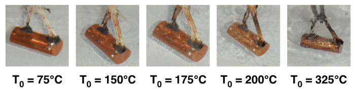
This experiment requires open-flame heating so before you begin ensure that a fire extinguisher is on hand and that no flammable materials are nearby. Follow all standard precautions for fire safety. Set up the burner near the quenching bath and light the flame. Pick up the test piece by the thermal cupel leads and from a safe holding distance, gradually heat it over the flame until it reaches the desired temperature. Now start the data acquisition and immerse the test piece into the quenching bath. Hold the piece as steady as possible to minimize heat transfer by forced convection. While the sample is cooling, watch for and note any boiling behavior. When the sample temperature drops to within a few degrees of the bath temperature, stop the data acquisition program. Repeat this procedure for progressively higher initial sample temperatures up to around 300 degrees Celsius.
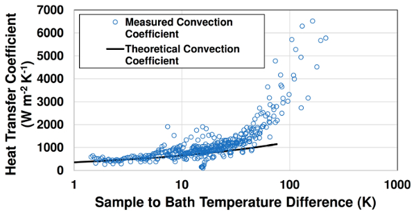
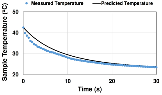
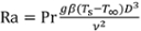
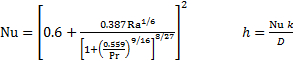
Open one of the data files. At every time step, there is one reading of the bath temperature and two of the sample temperature. Perform the following calculations for each time. Compute the average sample temperature by taking the arithmetic mean of the two sample readings. Calculate the instantaneous cooling rate which is the change in temperature divided by the change in time between two successive measurements. Then smooth the results with a two-point moving average to filter out some of the measurement noise. Use the differential equation derived from the lumped capacitance analysis to calculate the instantaneous heat transfer coefficient. The heat transfer coefficient can also be predicted using theoretical or empirical derived heat transfer models. These models generally report the convection coefficient in terms of the Nusselt number, a non-dimensional quantity. Consult the text for details on how to perform this calculation. With the equations for the theoretical heat transfer coefficient, you can also predict the sample cooling over time. To do this, take a starting point from your experimental data where the sample temperature is below 100 degrees Celsius. Choose a small numerical time step and assume that the bath temperature remains constant. Now, numerically integrate the differential equation from the lumped capacitance analysis. Soon, we will compare this theoretical prediction with our measurements. After you repeat this analysis for every data file, you are ready to look at the results. Plot the sample temperature versus time for a single test along with the theoretical prediction. The faster initial cooling rate is likely due to the forced convection as the sample is dropped into the bath. And later oscillations might be caused by small motions from the person holding the sample. Since the temperature prediction is soon set only free convection occurs, it is better to initialize the integration from a point after the forced convection stops. When this step is taken, the theory very accurately predicts how the sample cools over time. Now, plot the heat transfer coefficient against the sample to bath temperature difference for all of the tests together. Add the theoretical prediction for the heat transfer coefficient below the boiling point. Note the sharp rise at higher sample temperatures as the boiling process becomes more vigorous. In this experiment only boiling enhancement is observed. The low bulk fluid temperature in this case, prevents the onset of a boiling crisis.
Now that you are more familiar with the quenching process, let’s look at some ways in which it is applied in the real world. Heat treatment such as quenching and annealing are critical steps in the manufacture of durable tooling. Certain steel alloys can be annealed to reduce hardness for machining and working. Once formed, they can then be quenched to achieve high hardness. Many engineered components, such as computer processors, experience large temperature fluctuation throughout their life cycle. Processors heat up rapidly when running computationally intensive programs and the temperature rise triggers increased fan speeds to enhance cooling. The prediction and characterization of heat transfer rates is important for designing components that won’t fail due to overheating or fatigue.
You’ve just watched Jove’s Introduction to Quenching. You should now understand how this common heat treatment is performed as well as some of the major factors that effect heat transfer during the quenching process. You should also know how to perform a lump capacitance analysis to predict the change in temperature and how to use the Biot number to determine when this analysis is justified. Thanks for watching.
 (4)
(4) (5)
(5)