Turbulent flows play an important role in a wide variety of engineered and naturally-occurring systems. As a result, it is often necessary to perform measurements within the system in order to characterize the flow. Turbulent flows exhibit very high frequency fluctuations so any instrument that is used to measure and characterize turbulence must have a high enough time resolution to resolve these changes. Hot wire anemometers are often used for these measurements because they are small, robust, and fast enough to yield useful results. This video will illustrate how to use a calibrated hot wire anemometer probe to obtain velocity and turbulence measurements at different positions within a free jet and then perform a basic statistical analysis of the data to characterize the turbulent field.
A turbulent flow can be evidenced by high random fluctuations in flow variables such as velocity, pressure, and vorticity. These fluctuations are the result of nonlinear interactions between coherent motions within the flow field so the high frequency oscillations seen in measurements of turbulence are from real physical effects and not the result of random electronic noise. A classical description of turbulent flow involves the determination of the average value of flow variables and their corresponding fluctuations with time. For example, the average velocity, denoted by an over bar, is found by integrating the instantaneous velocity over the measurement time and scaling by the size of the integration domain. In the case of discrete measurements such as those from digital acquisition systems, the integral must be solved numerically. Once the average velocity has been found, it can be subtracted from the original signal to yield the time-dependent fluctuation and velocity denoted by the prime. From these definitions, it is easy to show that the average of a fluctuation field is zero. As a result, a more appropriate statistical descriptor for the fluctuation field is needed. A very common measure is the Root Mean Square or RMS of the fluctuations. This metric is similar to the average, except that the variable is squared before integrating and the square root of the result is taken. The turbulence intensity is given by the RMS of the velocity and this measurement will be demonstrated on a free jet in the next section. The average velocity of a free jet has an initially flat-top profile that smooths out as the jet propagates due to entrainment of surrounding air into the jet. This entrainment also causes the linear momentum of the jet to spread span-wise as the jet flows downstream resulting in widening of the jet as it propagates. The region of interaction between the jet and surrounding air is called the mixing layer and this region grows towards the center line as the jet moves downstream. This leaves a region inside the jet known as the potential core that is delimited in the stream-wise direction by the jet exit and the point at which the mixing layer reaches the center line. The potential core is then a region that has not been affected by interactions with the surrounding environment. On the center line, the potential core extends downstream to about four times the width of the jet exit. Now that you are familiar with the basics of turbulence measurements, let’s look at how this can be used to characterize a free jet.
Before you begin setting up, familiarize yourself with the layout and safety procedures of the facility. This experiment will be performed on the same flow system that was used for the hot wire anemometer calibration and the data acquisition system should be setup in the same manner. In the data acquisition software, set the sampling rate to 500 Hertz and the total samples to 5,000. Update the constants n, A, and B to match the values determined from the calibration. Now set up the flow facility. Use a calibrated spacer to set the slit width to 19.05 millimeters or three-quarters of an inch and then translate the hot wire anemometer to the vena contracta of the jet 1.5 times the slit width away from the exit. Starting with the anemometer above the slit, lower the height until the signal on the oscilloscope reaches a minimum fluctuation. Record this vertical position which corresponds to the center line of the jet. Now translate the anemometer back up until the signal fluctuation is a maximum and this position corresponds to the upper shear layer of the jet. Insert the blank orifice plate into the stack so that the flow velocity will be maximized and then turn on the flow facility. Once steady flow is established, use the data acquisition system to measure the average velocity and turbulence intensity at this point in the jet and record these values. Now move the anemometer span-wise down by two millimeters and measure the average velocity and turbulence intensity again. Continue lowering the anemometer by two millimeter increments and taking measurements until there is no noticeable change in both measurements. After recording the final height, translate the anemometer down until it is below the center line by the same distance. Resume taking measurements and translating up until the anemometer is back at the center line. When you are finished, translate the anemometer downstream until it is three times the slit width from the jet exit. Take measurements of the jet profile at this new stream-wise position following the same procedure you used in the first location. Repeat your measurements of the jet profile at six and nine times the slit width from the jet exit. After you’ve completed the measurements, shut down the flow facility.
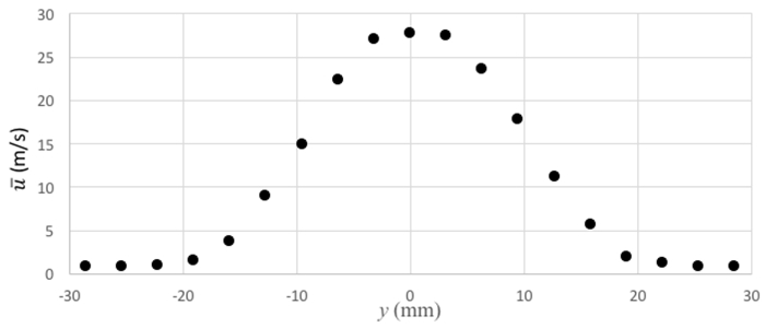
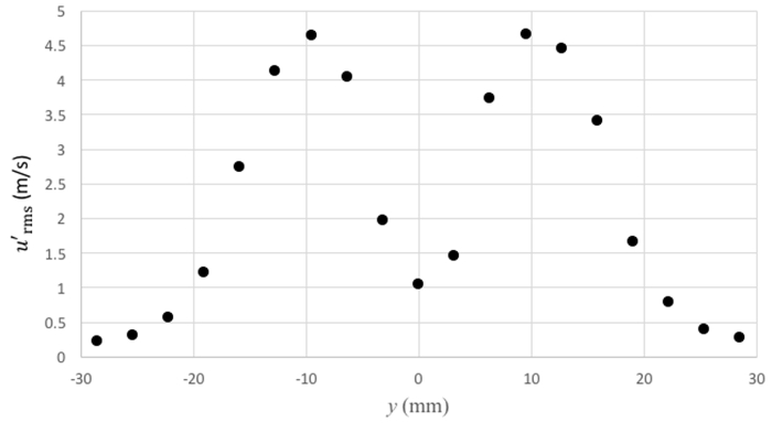
Take a look at your data. At each stream-wise position, you have measurements of the average velocity and the turbulence intensity taken at a series of span-wise points. First plot the average velocity as a function of the span-wise position. Scale the values by the center line value and find the points where the curve intersects the 50% threshold, interpolating as necessary. These points define the jet width Delta at this stream-wise position. Calculate the width by taking the difference. In this case, the width is about 21.5 millimeters. Now compare the average center line velocity and jet width at the different stream line positions. The center line velocity remains basically unchanged up to about four times the slit width from the exit due to the potential core, but decreases beyond this distance. The increase in jet width with distance is indicative of the span-wise spread of the linear momentum of the jet as the surrounding air is entrained. Now plot the turbulence intensity as a function of the span-wise position. Since mixing happens at the boundary between the jet and the surrounding environment, turbulence intensity peaks away from the center line.
Turbulent flow is ubiquitous in scientific and engineering applications. For its assessment in engineering applications such as ventilation, heating, and air conditioning, it is common to use portable hot wire probes that are introduced to the ducting and traverse radially to obtain the velocity profiles. This information is then used by the engineer to either balance a newly-installed flow system to ensure its proper operation or to troubleshoot a malfunctioning system and solve any problem that hinders its operation. When a new terrestrial, aerial, or marine vehicle or structure is designed to stand the forces of turbulent flows, it is necessary to test its performance under realistic flow conditions in a wind or water tunnel. To simulate turbulence conditions that occur in the atmosphere or ocean, the incoming flow can be disturbed with active or passive grids that will introduce significant fluctuations in the flow. Then the vehicle or structure under study can be mounted in the test section of the wind or water tunnel to measure how it copes with the loads introduced by the turbulent flow. These measurements can be made directly with aerodynamic balances that measure the resulting drag and lift forces. Also, the velocity around the model tested in the tunnel might give important information regarding performance. This characterization is typically made with hot wire anemometers in wind tunnels.
You’ve just watched Jove’s introduction to measuring turbulent flows. You should now understand how to deploy hot wire anemometers to measure and assess flow profiles and turbulence intensity. Thanks for watching.
 , which is defined as the distance between the two positions at which the local velocity is 50% of the centerline velocity. Note from table 2 that these two positions are somewhere in the intervals
  and
and 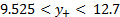 . Their exact locations are determined using linear interpolation, and are determined to be:
  mm and
  mm, for a jet thickness of
 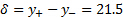 mm.
mm. , remains basically unchanged for
  , but decreases with
  for
for  . This effect is the result of the presence of the potential core for
  , and its disappearance for
  . The potential core is the region inside the jet that has not been affected by the interaction between the environment and the jet. The region of interaction is called the mixing layer, and it grows toward the centerline and away from the jet as the jet moves downstream. This growth is due to entrainment of surrounding air into the jet. Due to this entrainment effect, the linear momentum of the jet spreads in the spanwise direction, causing its width to increase with
  ) away from the centerline, at spanwise positions defined by
  and
and  . For simplicity, Table 2 only shows the values for the peak of turbulence intensity at the positive side of the jet.