Réseaux de canalisations et pertes de charge
English
소셜에 공유하기
개요
Source : Alexander S Rattner, département de génie mécanique et nucléaire, la Pennsylvania State University, University Park, PA
Cette expérience a introduit la mesure et la modélisation des pertes de charge dans les réseaux de canalisations et systèmes d’écoulement interne. Dans de tels systèmes, résistance à l’écoulement par frottement des parois du canal, raccords et obstruction provoque l’énergie mécanique sous forme de pression du fluide à être convertie en chaleur. Analyses de génie sont nécessaires au matériel de flux de taille pour s’assurer que les pertes de charge par frottement acceptable et sélectionner les pompes qui répondent aux exigences de baisse de pression.
Dans cette expérience, un réseau de tuyauterie est construit avec des caractéristiques communes de flux : longueurs droites de tubes, bobines de tube hélicoïdal et raccords coudés (coudes pointus de 90°). Mesures de perte de pression sont prélevés sur chaque ensemble de composants à l’aide de manomètres – simples dispositifs qui mesurent la pression du liquide par le niveau du liquide dans une colonne verticale ouverte. Les courbes de perte de pression qui en résulte sont comparés avec les prédictions des modèles d’écoulement interne.
Principles
Procedure
Results
Measured friction factor and equivalent length data are presented in Fig. 3a-c. For the straight tube section, a clear PVC tube with D = 6.4 mm and L = 284 mm is used. Measured flow rates (0.75 – 2.10 l min-1) correspond to turbulent conditions (Re = 2600 – 7300). Friction factors match predictions from the analytic model to within experimental uncertainty. Relatively high f uncertainty is found at low flow rates due to the limited accuracy of the selected (low-cost) flow meter (± 0.15 l min-1).
Friction factor results for the tube coil case also match the provided correlation (Eqn. 4) within experimental uncertainty (Fig. 3b). Five coil loops of radius R = 33 mm with tube inner diameter D = 6.4 mm are employed. Here, the Dean number is 500 – 5600, which corresponds to the laminar portion of Eqn. 4. Measured friction factors are significantly higher than for the straight section at equal flow rates. This stems from the stabilizing effect of the coil tube geometry, which delays the transition to turbulence to high Re.
For the elbow case, 4 elbow fittings (part number in materials list) are employed, connected by short lengths of D = 6.4 mm tubing. The equivalent frictional length of each elbow fitting approaches (Le/D) ~ 30 – 40 at high Re (Fig. 3c). This is similar to a commonly reported value of 30. Note that the actual frictional resistance is specific to the fitting geometry, and reported Le/D values should only be considered as guidelines.
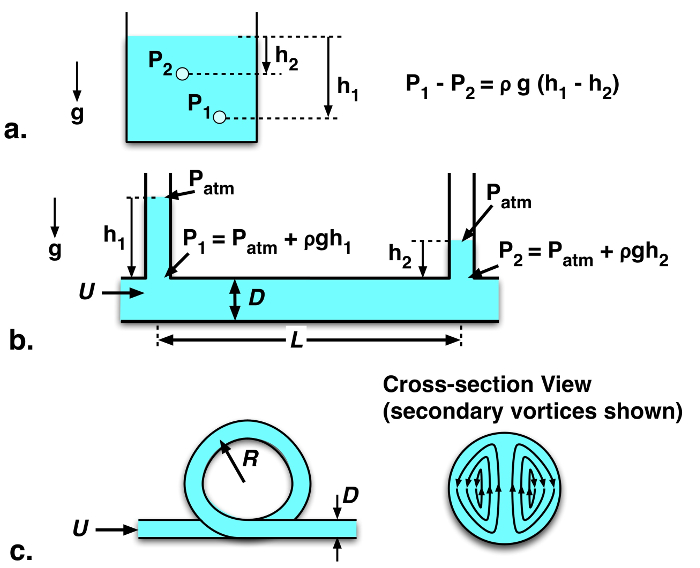
Figure 1: a. Schematic of hydrostatic pressure variation in a stationary body of fluid. b. Pressure change along a straight length of tube, measured with open-top manometers. c. Schematic of coiled tube, with internal vortices indicated in cross-section view.
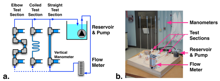
Figure 2: (a) Schematic and (b) photograph of pressure drop measurement facility. Please click here to view a larger version of this figure.
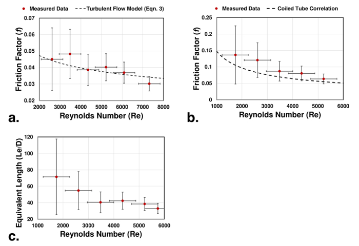
Figure 3: Friction factor and equivalent length measurements and model predictions for: a. Straight tube, b. Coiled tube, c. Elbow fittings.
Applications and Summary
Summary
This experiment demonstrates methods for measuring pressure-drop friction factors and equivalent lengths in internal flow networks. Modeling methods are presented for common flow configurations, including straight tubes, coiled tubes, and pipe fittings. These experimental and analysis techniques are key engineering tools for the design of fluid flow systems.
Applications
Internal flow networks arise in numerous applications including power generation plants, chemical processing, flow distribution inside heat exchangers, and blood circulation in organisms. In all cases, it is critical to be able to predict and model pressure losses and pumping requirements. Such flow systems can be decomposed into sections of straight and curved channels, connected by fittings or junctions. By applying friction factor and minor loss models to such components, whole network descriptions can be formulated.
Materials List
| Name | Company | Catalog Number | Comments |
| Equipment | |||
| Submersible water pump | Uniclife | B018726M9K | |
| Covered plastic container | Water reservoir, plastic food container used in this study. | ||
| Water flow meter | UXCell | LZM-15 | Rotameter, 0.5 – 4.0 l min–1 |
| Rigid clear PVC tube | McMaster | 53945K13 | For test sections and manometers, 1/4” ID, 3/8” OD |
| Flexible soft PVC tubing | McMaster | 5233K63
5233K56 |
For tubing connections and coil test section |
| Plastic tube fitting tee | McMaster | 5016K744 | For test sections inlet and outlet connections/manometers |
| Plastic tube fitting elbow | McMaster | 5016K133 | For test section with elbows |
References
- Perry, D.W. Green, J.O. Maloney, Perry's Chemical Engineers' Handbook, 6th Editio, McGraw-Hill, New York, NY, 1984.
내레이션 대본
Piping networks are commonly found in engineered and natural systems since they can efficiently transport, circulate, and distribute fluids. The water that comes out of the tap at your home travels through a complex city water supply system which is an excellent example of an engineered piping network. As fluid circulates through a piping network, it encounters frictional resistance from the channel walls and fittings and the fluid stream loses pressure as it overcomes these flow resistances. Characterizing and understanding these pressure losses is necessary to specify the correct components and sizes in a new design or to diagnose problems in an existing system. In this video, we will illustrate a simple approach for measuring the pressure drop within a pipe network and discuss some standard models for predicting losses and a few common geometries. Afterwards, these methods will be employed to experimentally measure pressure losses for comparison with the models. Finally, we’ll discuss a few other applications of piping networks and pressure losses.
Any time a fluid flows through a closed channel, it encounters some frictional resistance from the channel walls. As a consequence, a fraction of the fluid’s mechanical energy is converted to heat, resulting in a continuous loss of pressure in the direction of flow. This pressure loss can be characterized in a given system by measuring the fluid pressure at discrete points along the channel which is often done using simple liquid level devices called manometers. A manometer is an open vertical or inclined section of tube connected to the piping channel so that it partially fills with liquid. The height of the liquid column is directly proportional to the fluid level at that point along the channel. Therefore, the difference in pressure between two points or Delta P can be determined from the change in liquid height or Delta H between two manometers. Unfortunately, it is not always practical to make direct measurements and pressure losses must often be predicted before a system is built to ensure adequate fluid flow rates. In these situations, the Darcy Friction Factor formula can be used to predict frictional pressure loss. In this equation, Delta P is the pressure loss over a length L for a channel with a circular cross-section and an internal diameter D, row is the fluid density, and U is the average flow velocity, defined as the volume flow rate divided by the cross-sectional area of the channel, f is the Darcy Friction Factor which follows different empirically and theoretically-derived trends based on the Reynolds number and channel geometry. Refer to the text for the models used for straight circular channels and helical coils. The various channel sections in a pipe network are connected by discrete fittings such as valves, expanders, and bends that also contribute to pressure loss. The pressure losses through these fittings are known as minor losses and are sometimes reported in terms of the equivalent length of a straight channel required to yield the same pressure drop. These losses are still modeled with the Darcy Friction Factor formula using the friction factor and flow velocity of the connecting channels and the tabulated value of equivalent length scaled by the inner diameter for the fitting. Total losses in the piping system are simply the summation of all the losses from individual sections and fittings. In the following section, we will measure these losses in different representative pipe configurations to determine the friction factors and equivalent lengths.
Before you begin setting up, make sure that you have a clear area to work and a flat surface upon which to assemble the components. Affix the water reservoir to the surface and if necessary, drill holes for water inlet and outlet as well as the pump power cable. Mount the submersible pump in the reservoir. Now attach a small vertical beam or L bracket near the reservoir. Mount the rotameter flow meter vertically on the beam and use a section of tube to connect the pump outlet to the rotameter inlet. The rotameter is an instrument that indicates the volumetric flow rate of a fluid based on the floating level of a small bead. Construct the three-pipe test sections as described in the text. When you are finished, you should have a straight section, a coiled section, and a section with multiple elbow bends. Carefully record the lengths of any straight sections as well as the radius of the tube coil measured from the central axis of the coil to the midpoint of the tube. Mount all three sections to the surface with pipe clamps. Adjust the T fittings on the ends so that the branching side ports point up and then install clear ridged tubes on these ports to form the manometers. Use a level to ensure that the manometer tubes are vertical. Finally, connect one section of the tube to the outlet of the rotameter and place a second tube returning to the reservoir. These two tubes will connect to the inputs and outputs of the test sections to form a complete loop during the experiment. Fill the reservoir with water and the preparation is complete.
Connect the tube from the rotameter output to one end of the straight test section and connect the return tube to the other end. Now turn on the pump and adjust the rotameter valve to maximize the flow rate. Once all of the air is forced out of the pipe loop, turn off the pump. You may need to add additional water to the reservoir once the flow loop is filled. Once all of the air is forced out of the pipe loop, turn off the pump and compare the height of the water in the two manometers, measuring from the top of the T fitting. If the two heights are different, use shims to level the test surface until the measured heights are the same. Turn the pump back on and after waiting a moment for the flow to settle, record the flow rate and the vertical water level in both manometer tubes. Now adjust the rotameter valve to restrict the flow slightly and record the new flow rate and manometer levels. Repeat this procedure to gather data at six or seven flow rates for the straight test section. When you finish, repeat the experiment with the other two test sections including a readjustment of the test surface for each new section if necessary.
First, look at your data for the straight test section. At each flow rate, you have measurements for the water height in each manometer. Use the difference in manometer heights to determine the total pressure drop in the test section. Then determine the average flow velocity in the tube by dividing the flow rate measured from the rotameter by the cross-sectional area of the tube. Next, calculate the Reynolds number for the flow at this flow rate. Combine your results with the Darcy Friction Factor formula and your measurements of the test section to solve for the friction factor. For a straight section of length 284 millimeters and inner diameter of 6.4 millimeters, the measured flow rates from three-quarters to two liters per minute correspond to turbulent conditions. Propagate uncertainties to determine the total uncertainty in the Reynolds number and the friction factor as described in the text and then plot the result along with the model prediction for a straight section. Within experimental uncertainty, the friction factors matched the prediction of the model. The relatively high uncertainty in the friction factor at low flow rates is due to the limited accuracy of the flow meter. Now look at your data for the coiled test section. As before, determine the total pressure drop, average flow velocity, and Reynolds number at each flow rate. The total pressure drop in this section is the sum of the drop from the straight portion and the coiled portion so use the Darcy Friction Factor formula and the straight channel model to estimate the contribution from the straight section and subtract this from the total. Use the remaining pressure drop and your measurement of the coil radius to determine the friction factor in the coiled portion. Propagate uncertainties for the Reynolds number and friction factor once again, assuming negligible uncertainty from the correction for the straight section. Plot these results along with the model prediction for a coiled section. The Reynolds number is between 1,700 and 5,200 which corresponds to Dean numbers between 500 and 1,600 with the given tube diameter and coil radius. These values are within the Laminar portion of the coil friction factor formula. These measured friction factors also match the model within experimental uncertainty and for a given flow rate are significantly higher than those found in the straight section. This increases due to the stabilizing effect of the coiled tube geometry which delays the transition to turbulent flow to higher Reynolds numbers, about 9,900 for this geometry. Now take a look at the data for the third test section. Once again, determine the total pressure drop, average flow velocity, and Reynolds number at each flow rate. The total pressure drop in this section is due to the sum of the straight sections and minor losses from each of the N elbows. Use the Darcy Friction Factor formula and the straight channel model again to estimate and subtract the contribution from the straight sections. The remaining pressure drop is due to the N elbow fittings in the test section. Use this pressure drop with the friction factor and diameter of the straight sections to calculate the equivalent length for an individual elbow fitting. Propagate uncertainties for the Reynolds number and the equivalent length and plot your results. As the Reynolds number increases, the ratio of the equivalent length to internal pipe diameter approaches 30 as expected from the tabulate values. Note that the actual frictional resistance is specific to the fitting geometry and so these tabulated values should only be considered as guidelines.
Now that you are more familiar with pipe networks and pressure losses, let’s look at some real-world applications of these concepts. Heat exchangers typically consist of two separate piping networks that bring hot and cold fluid in close thermal contact without allowing them to mix. Pressure drop analysis must be performed when designing heat exchangers to ensure that the pumps can provide sufficient fluid flow rates and achieve the desired rate of heat transfer. Plaque buildup in arteries reduces the effective diameter for blood to flow. As a result, the heart has to work harder to compensate for the additional pressure loss. In extreme cases, the buildup increases the risk of a total blockage of the artery or heart failure. During an angioplasty procedure, a stent is inserted to re-expand the artery and restore normal blood flow.
You’ve just watched Jove’s introduction to piping networks and pressure losses. You should now understand how to determine pressure losses in a pipe network using the Darcy Friction Factor formula including the minor losses from discrete fittings. Finally, you have seen how to experimentally determine the pressure loss through a channel using manometer tubes. Thanks for watching.