1. Setup Layout and Alignment
- Installation and collimation of the tracking excitation laser
- Affix the laser to the optical table using a home-built mount. The mount is a simple aluminum plate with mounting holes for the laser head and the optical table. The laser should be firmly attached to a metal mount for stability and heat dissipation. For this work, use a 488 nm solid state laser for illumination (Figure 1), though the wavelength can be selected to suit a particular fluorophore or experiment. A critical factor is that the laser wavelength fit the 2D-EOD working range, which is determined primarily by the wave plate between the two deflectors (Figure 1: W2). The 488 nm laser can effectively excite the green or yellow fluorescent protein (GFP/YFP), which are common fluorescent tags in live cell experiments.
- Adjust the laser beam height and direction using a pair of dielectric mirrors (Figure 1: M). Make sure the laser beam is parallel to the optical table and adjust it to a suitable height.
NOTE: The height should be chosen based on the microscope platform. This height should be maintained for all subsequent mirrors used in this protocol, though it will not be explicitly stated. - Collimate the beam with a pair of lenses (Figure 1: L1 and L2). The focal lengths of lenses should be carefully chosen to avoid the laser spot being clipped by the aperture of the 2D-EOD. Clipping is evident by a change in the laser beam shape after passing through the 2D-EOD. The quality of collimation here is very important because aberrations will be amplified by subsequent lenses and any divergence will deteriorate the performance of the 2D-EOD deflection. Ideally, collimate the beam by focusing the beam to a point at least 20 m away.
- Place a pinhole (Figure 1: PH) of appropriate size at the focus of the first collimation lens (Figure 1: L1).
- Choose an appropriately sized pinhole. The pinhole size can be chosen based on the following calculation:
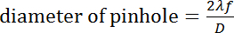
Where λ is the wavelength of laser, f is the focal length of the first lens, and D is the input beam diameter. - Mount the pinhole on a 3D translation stage so that it can be placed precisely at the focus of the first collimation lens.
- Adjust the position of the pinhole. Place a laser power meter after the pinhole and adjust the pinhole position in XYZ to maximize the power meter readout. If a diffraction ring is observed, block it with an iris placed before the 2D-EOD.
- Choose an appropriately sized pinhole. The pinhole size can be chosen based on the following calculation:
- Installation of Glan-Thompson polarizer
- Put the Glan-Thompson polarizer (Figure 1: GP) after the second collimation lens (Figure 1: L2) to clean the polarization of the laser beam. Rotate the polarizer to find maximum transmission with the power meter.
- Installation of EODs
- Use 2 EODs (Figure 1: EOD1 & EOD2) to deflect the laser in the X and Y directions. Maximize the laser transmission by adjusting the yaw, pitch, and height of each EOD.
- Align the two EODs with respect to each other using the alignment marker provided by the manufacturer on the side of each deflector.
- Apply a test pattern to the controller of the 2D-EOD to inspect the output of the EOD. This can either be the knight's tour (Figure 2) via the FPGA described below or a simple sine wave provided by a function generator. For the best performance, the deflection by each deflector should be parallel to either the X or Y direction of the piezo nanopositioner. This direction is dictated by the angular direction of the deflectors about the transmission axis. To rotate the deflection direction without moving the 2D-EOD, place a dove prism after the 2D-EOD to align the deflection axes to the piezo nanopositioner axes.
- Installation of half-wave plate
- Place a half-wave plate (Figure 1: W1) between the Glan-Thompson polarizer (Figure 1: GP) and the 2D-EOD to align the incoming laser beam polarization with the deflection axes of the 2D-EOD. Place a long focal lens (300 mm) after the 2D-EOD and place a sCMOS camera at the laser focus. Next, turn on the 2D-EOD to generate the knight's tour described below (Figure 2). Rotate the half-wave plate until an evenly square laser distribution is observed on the camera.
- Installation of a beam expending lens pair and relay lens pair
- Place a pair of lenses (Figure 1: L3 and L4) after the 2D-EOD to expand the beam to fill the back aperture of the objective lens (Figure 1: OL) and another pair of lenses (Figure 1: L5 and L6) to relay the focal plane to the microscope objective. Be sure to leave enough room between these two pairs of lenses as the TAG lens will be installed between them in a later step.
- Install the dichroic filter, 10/90 beam splitter, focusing lens, APD, objective lens, and fluorescence emission filter to complete the detection pathway.
- Install the dichroic filter (Figure 1: DC) to reflect the laser towards the objective lens. Align the laser to go straight through the center of the objective lens using two irises on the top and bottom of a long lens tube.
- Install a 10/90 beam splitter (Figure 1: BS) by which 10% of light is reflected for imaging by an sCMOS camera (described below) and 90% of passes through to the APD for tracking.
- Align the APD. Focus the laser onto a coverslip by the objective lens. Use the reflection from the coverslip to align all downstream elements by putting a coverslip at the objective focus and checking the intensity of the APD readout. After the beam splitter, install the APD focusing lens (Figure 1: L7) followed by the APD on a 3D translation stage. Position the lens such that the laser reflection from the objective goes through the center of the lens. The APD position can be optimized by adjusting the 3D position to maximize the intensity from the laser reflection on the coverslip. The APD position is at the optimal position when a move of the detector position in any direction decreases the intensity.
- Install a longpass fluorescence emission filter (Figure 1: F) before the beam splitter to remove the reflected and scattered light.
- Installation of the TAG lens
- Place the TAG lens between the two pairs of lenses (between Figure 1: L4 and L5) as mentioned before and shown in Figure 1. Adjust the yaw, pitch, height, and lateral position such that the beam passes perpendicularly through the center of TAG lens.
2. Sample Preparation.
- Fixed particle preparation
- Dilute 190 nm fluorescent beads to ~ 5 × 10⁸ beads/mL in PBS. Add 400 µL beads solution onto a coverslip and mount on the sample holder of the piezoelectric stage (the volume of beads will depend on the sample holder; the diameter of the sample holder chamber used here is 18 mm). For the beads used here, PBS causes the particles to deposit on the coverslip.
- Free moving particle preparation
- Dilute 110 nm fluorescent beads to ~ 5 × 10⁸ beads/mL with DI water. Add 400 µL beads solution onto a coverslip and mount onto the sample holder of the piezoelectric stage.
3. Optimize Tracking Parameters
- Raster scan fixed particles
- Put a fixed particle sample on the microscope.
- Turn on the laser, micropositioner controller, piezo nanopositioner controller, TAG lens controller, and EOD controller. Note that the order is not critical. Run the piezo nanopositioner in closed loop.
- Raster scan the sample in XYZ using a custom scanning software program (Figure S3, software available upon request from the authors), which drives the 2D-EOD in a knight's tour (Figure 2), collects counts from the APD, drives the piezo nanopositioner, and performs position calculation (Figure S2). The step size is 40 nm and the scanning range is 2 µm.
- To place the coverslip at the focus of the objective, remove the fluorescence emission filter and use the reflection of the laser from the coverslip to maximize the signal intensity as a function of the Z position of the micropositioner. After placing the sample at the focal plane, place back the fluorescence emission filter.
- Open the scanning program. Set the scanning range and step size by typing the number in the 'start', 'finish', and 'step'. First set a large scanning range and step size to locate a particle (e.g., 10 x 10 µm range with 200 nm step size). After finding the particle, shrink the scanning range and decrease step size (e.g., 2 x 2 µm range with 100 nm step size). Click the 'scan' button to perform a 3D raster scan to find the fluorescent focus.
- TAG lens settings (see also Figure 3)
- Click on the TAG lens control software. Click 'connect', 'power on' sequentially.
- To change the output phase of the trigger signals, it is necessary to change the output trigger mode. First change the mode from 'RGB' to 'Multiplane' and then change it back. Now the phase can be changed (Figure 3b).
- Set the output phase to be 0 °, 90 °, and 270 °. While any three phases which cover the phase space can be used, these three are found to work well empirically (Figure 3c).
- Select the 68,500 Hz frequency setting.
- To find the optimal frequency it is often necessary to change the frequency search range. Click 'advanced', 'setting'. Change the 'Max. Freq(Hz)' of column 0 from 70,000 Hz to 71,500 Hz. This can be adjusted to whatever frequency range is appropriate. Click 'Save Calibration', 'Exit Calibration' (Figure 3d).
- To make the new calibration effective, switch the resonance to another frequency (for example, 189,150 Hz) and then switched back to the 68,500 Hz frequency setting (Figure 3e).
- Change the amplitude gradually to 35%. Click 'Lock Resonance'. After the frequency is locked, click 'Unlock Resonance' (Figure 3e). The TAG lens is ready to use now.
- To calibrate, change the parameters that are used in the estimation to make the estimated position equal to the real position, as shown in Figure 4e, f. Input the scanning range of x, y, and z and then click the 'scan' button to scan the sample in XYZ to move the particle through the moving laser spot. The position of the particle as it is scanned through the laser focus should agree with the estimated particle position determined by the position estimation loop (Figure S1). The relationship between the estimated position and real position (Figure 4d) can be extracted from estimated position images (Figure 4f). If the positions do not agree, adjust the values of laser position (ck) used in the position estimation loop (Figure S1).
- Align TAG lens
- When the TAG lens controller is off, the raster scanned particle images (described below) taken before installing TAG lens and after installing TAG lens should look identical. Next, perform fluorescent particle Z stack scanning by moving the objective with the z nanopositioner to tune the position and angle of TAG lens (Figure 4). Tune the position of the TAG lens until there is no drift in the particle images in XY plane along the Z direction, which is achieved when there is no change in the XY position of the particle as a function of the Z position (Figure 4d). The tracking system is ready to use after alignment of the TAG lens.
- Installation of sCMOS camera for particle monitoring
- Install a sCMOS camera to visualize particles while they are being tracked. Install the sCMOS only after the all the components of the tracking system have been installed and optimized. Load a fixed fluorescent particle sample onto the microscope and run the tracking program to lock one particle in the objective focal volume. Then, install the 100 mm focal length lens (Figure 1: L8) and sCMOS. Adjust the sCMOS position so that the image of the particle is focused to the smallest and brightest spot.
4. Real-time 3D Tracking of Freely Diffusing Nanoparticles
- Put the 110 nm free moving particle sample on the microscope.
- Turn on laser, micro-positioner controller, piezo nanopositioner controller, TAG lens controller, and EOD controller. Run the piezo nanopositioner in open loop. Set the TAG lens software according to step 3.2.
- Open and run the tracking software (available upon request from the authors). Set the position estimation parameters to their optimized values, which were found in Section 3.
- To place the coverslip at the focus of the objective, remove the fluorescence emission filter and use the reflection of the laser from the coverslip to maximize the signal intensity as a function of the Z position of the micropositioner. After finding the coverslip, increase the focus position 15 µm to focus the laser away from the coverslip and into the solution. Place back the fluorescence emission filter.
- Set the integral control constants. The integral control constants can be set starting at a low value and slowly increasing until oscillations can be seen in the particle's position readouts. Once oscillations are observed, set the integral control constants to 80% of the value causing the oscillations. Typical values will be around 0.012 for the XY 'integral gain' and 0.004 for the Z 'integral gain'.
- Set the tracking thresholds in 'Track Threshold' and 'Track Minimum' and start the tracking experiment by clicking 'Search' and 'Auto Track'. The threshold for terminating tracking is set slightly higher than the background level and the threshold for triggering tracking is about two times higher than the background. Here, the threshold for triggering tracking is 3 kHz and the threshold for ending the trajectory is 1.5 kHz.
Fixed particle scanning (Figure 4) and freely diffusing 110 nm fluorescent particle tracking (Figure 5) were performed following the protocol above. The particle scanning was performed by moving the piezoelectric nanopositioner and bin photons while simultaneously calculating the particle's estimated position at each point in the scan. The scanning image shows a square of even intensity (Figure 4a) and the estimated positions show a linear relationship with the particle's real position over a 1 × 1 × 2 µm range in x, y, and z direction (Figure 4b–f).
To demonstrate real-time tracking, 110 nm fluorescent particles were tracked in water by 3D-DyPLoT (Figure 5a, b). The mean square displacement (MSD) analysis shows a typical linear behavior characteristic of Brownian motion (Figure 5c). MSD analysis of 30 trajectories showed a mean hydrodynamic diameter of 110 nm, in good agreement with the manufacturers specification for the size of the fluorescent nanoparticles being tracked (Figure 5d). In addition, Movie 1 shows the real-time piezoelectric nanopositioner readouts and synchronized sCMOS images for a 2 min long trajectory of a freely diffusing 110 nm fluorescent particle.
In addition to being able to track with high speed, slow moving particles can be localized with high precision. Figure 6a–d shows the application of the 3D-DyPLoT system to fixed particles using the same feedback parameters as used for high speed tracking, showing a precision of 17.6, 26.4, and 53.4 nm in X, Y, and Z, respectively with photon count rate of 105. Figure 6e–h shows the precision under feedback control reduced by a factor of 10, effectively swapping speed for precision and exhibiting a precision of 6.5, 8.3, and 10.5 nm in X, Y and Z, respectively.
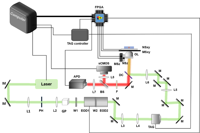
Figure 1. Schematic of 3D tracking system. The 2D-EOD (EOD1 & EOD2) and the TAG lens (TAG) deflect the laser along the XY and Z directions, respectively. The APD (APD) is used to collect fluorescence photons, which are sent to the FPGA (FPGA). FPGA is used for the position calculation algorithm, photon counting, control of the 2D-EOD as well as control and readout of piezoelectric nanopositioner (NSxy and NZz). Other components labeled in the figure: mirrors (M); lenses (L#); pinhole (PH); Glan-Thompson polarizer (GP); half-wave plate (W1); dichroic filter (DC); objective lens (OL, 100X NA = 1.49); fluorescence emission filter (F); beam splitter (BS); XY micropositioner stage (MSxy); Z micropositioner stage (MSz). Please click here to view a larger version of this figure.
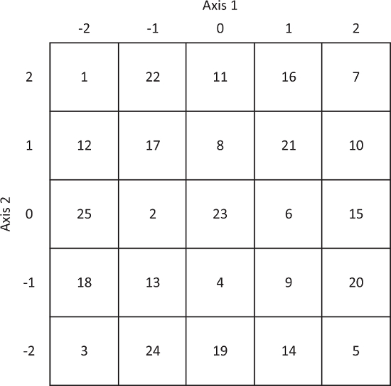
Figure 2. Coordinates for the knight's tour implemented in 3D-DyPLoT. Axis 1 and axis 2 should be aligned along the X or Y axis by proper alignment of the 2D-EOD. Please click here to view a larger version of this figure.
Figure 3. TAG lens software settings. See section 4.2 TAG lens settings for more information. Please click here to view a larger version of this figure.
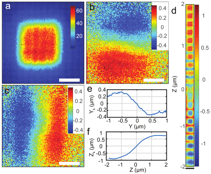
Figure 4. Particle scanning and position estimation. (a) Scanning image of 190 nm fluorescent beads with 2D-EOD driving the laser in a 1 × 1 µm square knight's tour pattern. Fluorescence intensity is denoted by color. Unit: kHz. (b) Estimation of xk, the particle's position relative to the center of the 2D-EOD scan in micrometers. The color in b, c, and d denotes the estimated position. Unit: µm. (c) Estimation of yk in micrometers. (d) Estimation of zk, the particle's position relative to the axial center of the TAG lens scan in micrometers. (e) Estimated particle position yk as a function of the stage position averaged over the entire grid from (c). Note that the estimated particle position acquired from the position estimation algorithm (yk) agrees with the real position. (f) Estimated particle position zk as a function of the stage position averaged over the entire grid from (d). The estimated position shows a linear relationship with particle's real position over 1 × 1 × 2 µm range in X, Y, and Z direction. Note that the estimated particle position acquired from the position estimation algorithm (zk) agrees with the real position. The estimated position shows a linear relationship with particle's real position over a 1 × 1 × 2 µm range in X, Y, and Z direction. The white scale bars in (a–c) represent 500 nm and the black scale bar in (d) represents 2 µm. Please click here to view a larger version of this figure.
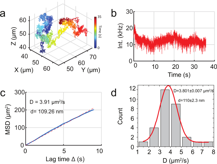
Figure 5. Tracking 110 nm fluorescent particles in water with 3D-DyPLOT. (a) 3D trajectory of a freely diffusing 110 nm fluorescent nanoparticle in water. (b) Fluorescent intensity as a function of time for the trajectory in (a). (c) MSD of the trajectory in (a). The blue line is the measured MSD while the dotted red line is best fit line from linear regression. (d) MSD analysis of 30 trajectories, showing a mean hydrodynamic diameter of 110 nm, in good agreement with the size of the fluorescent nanoparticles being tracked. The diameter of the particles was calculated using the Stokes-Einstein relation. Please click here to view a larger version of this figure.
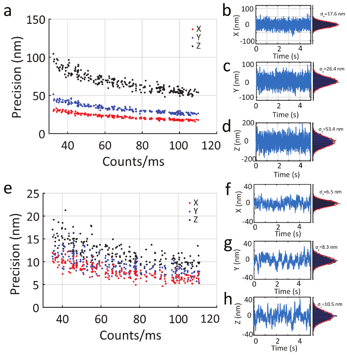
Figure 6. Precision of fixed particle tracking. (a) A fixed particle is tracked by 3D-DyPLoT at different count rates. The precision is (b) 17.6 nm in X, (c) 26.4 nm in Y, and (d) 53.4 nm in Z at an emission rate of 100 kHz. (e) When probing slower processes, the feedback control constant (KI) can be reduced by a factor of 10 to increase precision. Under this reduced feedback control, the precision is (f) 6.5 nm in X, (g) 8.3 nm in Y, and (h) 10.5 nm in Z at an emission rate of 100 kHz. Please click here to view a larger version of this figure.
Figure S1. Please click here to download this file.
Figure S2. Please click here to download this file.
Figure S3. Please click here to download this file.
Supplementary Information. Please click here to download this file.
Although many varieties of 3D single particle tracking methods have emerged in recent years, robust real-time tracking of high speed 3D diffusion at low photon count rates with a simple setup is still a challenge, which limits its application to important biological problems. The 3D-DyPLoT method described in this protocol addresses these challenges in a several ways. First, the excitation and detection pathways are simplified greatly compared to other implementations making alignment simple and robust. Secondly, the moving laser spot and position estimation algorithm provide precise position estimates for the feedback loop, making the feedback more stable. Thirdly, the effectively large detection range (1 x 1 x 4 µm) of the dynamically moving laser spot allows for tracking of fast moving particles. To see why this large detection area is critical, it is important to consider the intrinsic response time of the piezoelectric nanopositioner. High speed piezoelectric stages have resonances on the order of 1 kHz, limiting the response time to be on the order of 1 ms. In 1 ms, a 100 nm nanoparticle with a diffusion coefficient of 4 µm2/s, will diffuse on average 90 nm from the center of the diffraction-limited detection volume. This is only the average displacement and truly random motion will exhibit steps much larger than this, leading to the particle leaving the focal volume and ending the current trajectory. The situation is even worse for smaller particles, where increasingly larger thermal diffusive steps lead to loss of tracking. The effectively large detection area allows for the tracking system to overcome intrinsic piezoelectric stage lag and recover from large diffusive jumps in the particle position, increasing the overall robustness of the tracking mechanism. Finally, the large scan area allows the system to easily pick up new particles, allowing for consecutive trajectories to be rapidly acquired and large data sets compiled.
The user should keep in mind that there are some critical steps. First, the alignment of both the 2D-EOD and the TAG lens are critical. Both must be well aligned to obtain the optimum precision. Second, the parameters that are used in the position estimation in the fixed particle scanning step must be well calibrated (see Figure 4). The estimated particle position should match the particle position corresponding to the center of the laser scan range. Finally, the feedback integral constants (KI) should be tuned carefully, starting with a small value and then ramping up until oscillations are observed, then backing off to about 80% of that value.
There are a few caveats about 3D-DyPLoT to keep in mind depending on the desired application. While the optimized position estimation is designed for use with Brownian motion, it is also well suited towards directional motion. The algorithm can be directly applied to any type of motion since it is only the position uncertainty that is assumed to be Gaussian, not the real particle position. For cases where persistent linear motion is expected, an additional term can be added to the prediction term in the position estimation algorithm (see Equation 3 in the Supplementary Information).
The selection of the parameters for the 2D-EOD and TAG should be carefully considered when setting up the 3D-DyPLoT. Of particular importance is the bin time used for the knight's tour scanned by the 2D-EOD. In an ideal scenario, the knight's tour would be synchronized to the period of the TAG lens to ensure efficient sampling. However, it is critical to consider the response time of the 2D-EOD to step changes in voltage. For the unit used here, there is a 2-3 µs response time after the voltage is applied before the desired spot is reached. At 20 µs bin time, this is about 10-15% of the collection time. Reducing the time so that it matches the TAG lens period of ~ 14 µs increases the fraction of the bin time, which is the lag time of the 2D-EOD. This leads to incorrect values of the laser position and incorrect position estimates.
Another factor for the experimenter to keep in mind is temporal resolution. While the data shown here are collected at a 100 kHz data rate, the ultimate temporal resolution is defined ultimately by which data are used for the position measurement. If the readout of the nanopositioner is used as the particle position (Figure 6), the temporal resolution will depend on the value of the integral control constant. For example, for the integral control shown in Figure 6a–d, the stage response is on the order of 1 ms, while for Figure 6e–h, it is on the order of 10 ms. If faster temporal resolution is desired, then the photon-by-photon result of the position estimation algorithm will correlate with the photon count rate. For example, a 10 kHz emission rate yields 100 µs temporal resolution and a 100 kHz emission rate yields a 10 µs temporal resolution. In addition, since the precision follows a  relationship41, the spatial and temporal precision are coupled. As a result, the brightness of the probe determines both the spatial and temporal precision.
In this protocol we described the setup, layout, and alignment of a high speed real-time 3D single particle tracking method which utilizes a 2D-EOD and TAG lens to dynamically move a focused laser spot to achieve rapid particle position estimation. We then described sample preparation and parameter optimization methods. 3D-DyPLoT provides a robust and relatively simple method to lock-on to fast moving and lowly emitting diffusive particles. The simple optical layout allows it to be easily added onto the side-port of any existing microscope stand so that it might be combined with imaging modules. With this protocol, we hope that RT-3D-SPT can be more widely implemented by more investigators to address fast, three dimensional biological processes.
