Resistor ‘R’, inductor ‘L’, and capacitor ‘C’ are fundamental circuit elements, each with different properties that are the basis of all modern electrical devices.
A resistor is an electrical component that dissipates energy, usually in the form of heat. In contrast, a capacitor stores energy in an electric field, and an inductor stores energy in a magnetic field.
When resistors, capacitors and inductors are connected together, the circuits display time and frequency dependent responses useful for AC signal processing, radios, electrical filters and many other applications.
This video will illustrate the behaviors of a resistor-capacitor and a resistor-inductor circuit, and show the oscillation in an inductor-capacitor circuit with little resistive energy loss.
Let’s learn how current and voltage behave in circuits involving resistors, inductors and capacitors.
First, let’s talk about a circuit of a resistor in series with a capacitor, called an RC circuit. When the switch is closed, the output of the voltage source is applied across both components and current starts flowing. As, the capacitor is initially uncharged, it has zero voltage across its terminals. Hence, all of the voltage source’s output appears across the resistor and the current is at its maximum value.
If we look at the plot of voltage and current against time, initially VR equals source voltage the voltage across the capacitor ‘VC’ is zero and the current is at its max. As the current charges the capacitor, ‘VC’ increases. In response, VR decreases and therefore the current also goes down, in accordance with Ohm’s Law. Eventually the resistor voltage is zero and the current flow stops.
A similar analysis is possible for an RL circuit consisting of a resistor in series with an inductor. At the instant the switch closes, the sudden flow of charge creates a magnetic field in the inductor, and its voltage ‘VL’ is equal to the source’s voltage. Consequently, the initial VR is zero and thus the initial current is also zero.
Now, to monitor the changes, let’s look at the voltage and current graphs like before. Over time as the inductor voltage decreases, the voltage across the resistor increases and therefore the current also increases. Ultimately, the inductor voltage is zero, all of the voltage source output is across the resistor, and the current is at its maximum value.
The decay of current and voltage transients in RC and RL circuits is caused by energy dissipation in the resistor. In contrast, an LC circuit, which has a capacitor connected to an inductor, ideally has no resistance or energy loss, and exhibits very different behavior.
If the capacitor in this circuit is charged to voltage V and then connected to the inductor, electrical energy stored in the capacitor is transferred to the inductor and converted to magnetic energy. The inductor then transfers its energy back to the capacitor then the process reverses with the current flowing in the opposite direction, this process repeats indefinitely and the voltage across each component oscillates sinusoidally with time.
An RLC circuit like this one adds a resistor to the LC circuit. Oscillations in this configuration dampen because the resistor dissipates energy during each cycle. Eventually the oscillations stop when the voltage and current decay to zero.
Now that we’ve explained the basics of RC, RL and LC circuits, let’s take a look at their behaviors in the laboratory.
Obtain an oscilloscope, a small light bulb with a resistance of a few ohms, a switch and a DC voltage supply or 1.5 volt battery. Assemble this circuit and leave the switch open.
Select the vertical scale of the oscilloscope to 1 volt per division and the time scale to 1 second per division. Later it may be necessary to adjust these settings for optimal viewing of signals during the various tests.
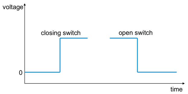
Close the switch to apply power to the light bulb.
Because the light bulb acts like a resistor, the current through it is proportional to voltage. As the oscilloscope traces show, the bulb brightens instantly when the switch closes and darkens instantly when the switch opens.
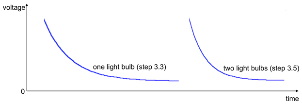
Assemble the circuit as shown with a 1 Farad capacitor in series with the light bulb. Note that the oscilloscope measures voltage across the resistor. Leave the switch open until the start of the test.
Close the switch and observe the light bulb and the oscilloscope trace. The light bulb glows briefly before darkening because the capacitor passes current when the voltage changes suddenly, when the switch closes. As time progresses, the current through the circuit decays due to the light bulb resistance and the capacitance.
Open the switch and modify the circuit by connecting a second light bulb in parallel with the first.
Again close the switch. Watch both light bulbs and the oscilloscope trace. The two parallel bulbs turn on and off more quickly than the single bulb. This is because the parallel resistance of two bulbs is smaller than the resistance of a single bulb. The resulting circuit has a shorter drop in the current and a faster response.
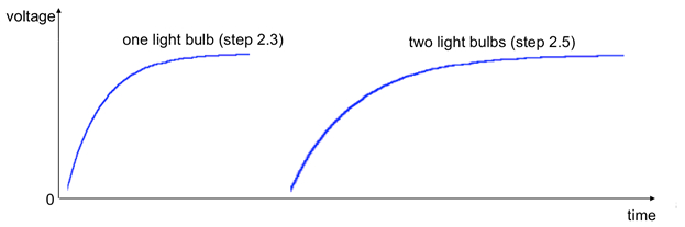
Assemble this circuit with a 1 milli Henry inductor in series with the light bulb. Leave the switch open until the start of the test.
Close the switch and observe the light bulb and the oscilloscope trace. The light bulb takes a small amount of time to turn on because the inductor conducts little current when the voltage changes suddenly, as when the switch closes.
As time progresses, the inductor’s current-and that through the bulb-approaches a steady state level. Open the switch and connect a second light bulb in parallel with the first.
Again close the switch. Watch both light bulbs and the oscilloscope trace. The two parallel bulbs turn on and off more slowly than the single bulb. This is because the parallel resistance of two bulbs is smaller than the resistance of a single bulb.
Assemble this circuit with a 10 micro Farad capacitor, and an 8 milli Henry inductor, along with the oscilloscope connected across the capacitor. Close switch 1 to charge the capacitor and leave switch 2 open until the start of the test.
Open switch 1 to disconnect the voltage source from the circuit. Close switch 2 and observe the oscilloscope. The inductor voltage oscillates and may show some damping caused by the small resistance of the wires in the circuit. The period of oscillation is on the order of milli seconds, which is consistent with the expected time based on the values of capacitance and resistance.
Resistors, capacitors and inductors are simple components but the RC, RL and LC circuits that use them have complex behaviors, which enable many applications in electronic signal processing, timing circuits, and filters.
In this example, researchers implanted subcutaneous radio transmitters in mice to study blood pressure as they moved freely. Radio receivers commonly use inductor-capacitor circuits to select a specific frequency from the broad band of intercepted radiofrequency, or RF, energy. The correct frequency carries the desired information for amplification and further processing by additional electronics in the receiver.
Electroencephalographs measure electrical activity in the brain. Electrodes placed over the scalp pick up millivolt level signals over a wide frequency range. RC, RL, and LC circuits are part of the filters that reduce electrical interference and artefacts, thus helping in acquisition of meaningful data.
You’ve just watched JoVE’s introduction to the time dependent behavior of circuits using resistors, capacitors and inductors. You should now understand the basics of RC, RL, and LC circuits, and how these circuits differ from one another. Thanks for watching!
 ) based on the values of capacitance and resistance.