Detection and Quantification of Nucleic Acids by Real Time PCR

English

Overview

Real Time PCR, or quantitative PCR (qPCR), is a technique used to measure the amount of nucleic acids, i.e. DNA or RNA, in a given sample. It can be used for myriad applications, such as measuring the levels of microorganisms in a sample, identification of transgenes in genetically modified food, and determining gene dosage or mRNA expression levels of genes of interest under different experimental conditions (Kubista et al., 2006).

qPCR, as conventional PCR, uses DNA as the template that will be amplified. When measuring differences in DNA content, the sample can be used directly. On the other hand, in order to measure RNA levels, qPCR requires an additional step. As DNA polymerases cannot directly bind and amplify RNA, samples must be converted to DNA. That process is known as reverse transcription (RT). RT is performed by an enzyme from viral origin called reverse transcriptase, which is able to bind single stranded RNA and synthetize single stranded complementary DNA (cDNA) (Alberts et al., 2014). The use of qPCR to measure RNA levels is known as reverse transcription quantitative PCR (RT-qPCR).

In order to quantify a sample, a short PCR target sequence within the area of interest is selected. Short target sequences increase the efficiency of the PCR and reduce the risk of amplifying non-specific PCR fragments that are typically longer. Real time PCR targets are amplified by a combination of specific sense (forward) and antisense (reverse) primers (short DNA oligonucleotides). Selection of good primers is key to a successful qPCR outcome (Bustin and Huggett, 2017; Thornton and Basu, 2011). When measuring RNA levels by RT-qPCR, it is preferred to select primers spanning over two or more introns, to hinder amplification of contaminating genomic DNA (gDNA). The PCR product from cDNA will be shorter and therefore will amplify much more efficiently than any long, intron-containing products from gDNA (Bustin and Huggett, 2017). If possible, primers are designed to bind exon-exon junctions, thereby preventing amplification of corresponding gDNA.

Since in RT-qPCR the total RNA levels might vary among samples, the levels of a PCR target of interest need to be normalized to a reference gene. The reference gene is selected based on its high and steady expression among all the studied cells and tissues, and across all experimental conditions. Reference genes typically are housekeeping genes, such as ribosomal proteins, actin, or tubulin (Ponton et al., 2011). However, depending on the experimental conditions, they can show unwanted variation in their expression (Ponton et al., 2011). Therefore, the first time an experiment is performed, it is recommended to test various reference genes to ensure they fulfill the premises from above.

The main difference of qPCR versus regular PCR is that the amount of DNA in the sample is measured in real time, after every amplification cycle (Kubista et al., 2006). During the qPCR run, the target is detected and quantified by measuring a fluorescence reporter that interacts with DNA (Wittwer et al.). The reporter can either be a DNA-binding dye, or a probe present in the reaction mixture. DNA-binding dyes are small molecules, such as SYBR Green, that will bind double-stranded DNA products. Once intercalated in the DNA, these dyes fluoresce when illuminated with UV light. These probes are molecules that specifically bind, and fluorescently label, the PCR product generated during the reaction. Probes hybridize to a unique DNA sequence, increasing the specificity of the qPCR, as only the specific PCR product will be fluorescently labeled. However, it also increases the costs, as one specific probe has to be designed for each target. Regardless of the method, the outcome is the same. Every PCR cycle the target DNA in the reaction is doubled. This in turn doubles the number of reporter molecules binding to the DNA. Following each cycle of DNA amplification, the PCR reaction is illuminated by a light source, eliciting a fluorescence signal from the reporter, which is detected by a sensor. Since the fluorescence signal is proportional to the amount of amplified PCR target, the measurement of fluorescence allows to quantify the relative amount of DNA.

After the qPCR run, DNA levels are calculated by comparing the cycle at which different samples reach a certain fluorescence intensity, which has to be set at the exponential increase of fluorescence. This threshold level will define the quantification cycle (Cq, previously also known as cycle threshold or Ct, crossing point or Cp, take-off point or TOP), which is the cycle at which a sample reaches the intensity threshold (Bustin et al., 2009). Every PCR cycle the DNA amount is doubled, providing the basis to calculate differences in DNA content based on the Cq from each sample. The most common approach to calculate these differences is the ΔΔCq method (Bustin et al., 2009). First, the differences between the target and the reference are calculated (ΔCq). This normalizes the DNA content among samples. Afterwards, the ΔCq of the different samples are compared directly, obtaining the ΔΔCq value. The differences in DNA are then calculated as 2-(ΔΔ^Cq).

In this protocol, we will quantify the differential gene expression of Drosocin, an antimicrobial peptide produced in response to bacterial infection, using Drosophila melanogaster as model organism. We will compare the levels of Drosocin expression in whole flies under three conditions, 6 hours after the challenge, typical for an infection experiment in innate immunity research.
– Control flies
– Flies injected with PBS (“sterile” or aseptic injury)
– Flies injected with Escherichia coli (bacterial infection or septic injury)

We will detect qPCR products by using DNA-binding dyes, and will use the ΔΔCq quantification. To normalize the RNA levels, we will use the ribosomal protein gene RpL32 as reference target.

Procedure

1. Experiment set-up

Select a PCR target sequence in the gene of interest and design primers to amplify a product of 70 to 150 bp length. Do the same for a reference gene whose expression levels are homogeneous in all samples. In our example we used the ribosomal protein gene RpL32. The primers used to analyze the levels of drosocin are listed below:
- – Drosocin Fwd: CCATCGTTTTCCTGCT
- - Drosocin Rev: CTTGAGTCAGGTGATCC
- - RpL32 Fwd: GACGCTTCAAGGGACAGTATCTG
- - RpL32 Rev: AAACGCGGTTCTGCATGAG
Combine the PCR primers in a single mixture containing 5 μM from each primer. Although this step is optional, it will simplify the pipetting afterwards.

Plan the PCR run. We recommend preparing a scheme for the desired PCR plate format (96-well or 384-well), noting which sample is run on each well. For each sample, 3 technical replicates (to account for pipetting or measuring errors) should be included. Also, a minus reverse transcriptase control per sample (RNA without reverse transcriptase reaction) should be included, in order to control for unwanted amplification of gDNA. In the analysis of Drosocin, samples were arranged in the following scheme in a 96-well qPCR plate:

RpL32 Uninjected`	RpL32 Uninjected	RpL32 Uninjected	Drosocin Uninjected	Dro Uninjected	Dro Uninjected
RpL32 PBS	RpL32 PBS	RpL32 PBS	Droscocin PBS	Droscocin PBS	Droscocin PBS
RpL32 E. coli	RpL32 E. coli	RpL32 E. coli	RpL32 E. coli	RpL32 E. coli	RpL32 E. coli

If it is the first time a qPCR for a particular gene of interest is run, prepare serial dilutions of the cDNA samples (1/10 and 1/100 of the already diluted sample, see below) to determine optimal sample concentration.
Configure the reaction protocol in the qPCR machine. To setup the qPCR, first use the “Setup” menu to define the experiment name and properties. Set the plate to a 96-well plate, choose SYBR as the detector, and select the ΔΔCt protocol. Then navigate to the next menu to set the qPCR targets and samples. Define the reference gene (RpL32) and the reference sample (Uninjected). Next, jump to the “Assign” tab to populate the plate information by assigning the specific sample and target information for each well. To finish programming the experiment, define the qPCR parameters in the “Method” menu as follows:
- 95ºC for 3 min (initial DNA denaturation)
- 40 cycles:
  - – 95ºC for 15 sec (denaturation)
  - – 60ºC for 1 min (annealing and extension)
- One cycle to calculate the melting curve (automatically defined by the instrument).

2. RNA extraction

Extract RNA from samples, using an RNA extraction kit/method following the manufacturers’ protocols. Try to maintain an RNase free environment by using gloves and a lab coat, barrier pipet tips, and clean work surfaces with an RNase-cleaning product.
Treat the samples with DNase when using qPCR primers that do not span introns. In our example, we extract RNA from 10 adult whole flies per sample.
Measure the RNA concentration and dilute all samples to the least concentrated sample with RNase-free H₂O, or to 1 μg, whichever is lower. Otherwise, varying cDNA content among samples might affect the qPCR results.
RNA can be stored at -80ºC for ~2 years.

3. cDNA preparation

Convert the RNA into cDNA by using a cDNA synthesis kit, following the manufacturer’s protocol. Typically, 10 ng to 1 µg of total RNA is used as input for the cDNA synthesis reaction
Dilute the resulting cDNA 1/10 with ddH₂O. Without dilution, the newly synthesized cDNA is usually too concentrated for qPCR
Note: If qPCR from DNA is performed, start with DNA extraction of the samples of choice, and measure DNA concentrations and adjust to the lowest concentrated sample or 100 ng, whichever is lower.

4. Assembling the qPCR

Label with a permanent marker the PCR plate according to the scheme prepared beforehand, to facilitate pipetting
Prepare a qPCR master-mix for each PCR target containing the Taq polymerase + fluorescent dye mix, PCR primers and ddH2O (See table 1).

Reagent	μl for 1 sample	µl for 15 samples
2x iTaq SYBR Green universal mix	5	80
10 μM forward primer	0.5	8
10 μM reverse primer	0.5	8
cDNA Template	2	32
ddH2O	2	32
Total	10	160

Table 1. qPCR reaction mix for each of the targets evaluated with the real time PCR.

Add 8 μl of qPCR master mix to each reaction well.
Add 2 μl of the cDNA template to each reaction well.
Include negative control samples (Mastermix without DNA and mastermix with RNA as template to account for genomic DNA contamination).
Carefully seal the plate with adhesive seal. Ensure each and every well is properly sealed to avoid evaporation of the samples or unwanted mixing, which would result in wrong measurements.
Vortex briefly the plate to properly mix the PCR components.
Centrifuge 10 sec the plate in a tabletop centrifuge to bring all the reaction volume to the bottom of the wells.
Place the qPCR plate in the machine and start the qPCR run as specified in step 1.5.

5. Analyzing the qPCR data using the comparative ΔΔCq method

Export the Cq values from the instrument by clicking the “Export” menu from the results panel. There is no need to change any of the default analysis parameters. Save the spreadsheet and, if needed, transfer it to a personal computer to continue with the RT-PCR analysis.
By using Excel or another compatible software, calculate the mean Cq and standard deviation for the 3 technical replicates from each sample. To do so, use the formulas AVERAGE and STDEV.S for the mean and the standard deviation respectively. Make sure that none of the technical replicates differs more than 1 Cq from the other two. These outliers should be discarded from the analysis. If this variation is observed among all technical replicates, the qPCR should be repeated, as it indicates pipetting or measurement errors.
Normalize the cDNA content of the samples to the reference gene by calculating the ΔCq for each sample, using the mean Cq calculated in the prior step as follows:
ΔCq = ΔCq(target) - ΔCq(Reference)
Calculate the ΔΔCq for each experimental sample against the control group:
ΔΔCq = ΔCq(experiment) - ΔCq(control)
Calculate the differences in RNA expression by using the following formula to calculate the fold change in cDNA among samples:
Fold change = 2^-(ΔΔCq)
Fold changes can be displayed in a table or a bar chart. Ideally, each experiment is performed in at least three biological replicates; of these data the mean and standard deviation (SD) are calculated and displayed.
To average several biological replicates, transform the fold changes into log2(fold changes) and use these values to calculate the mean and standard deviation of the biological replicates. The resulting values can be directly plotted, or they can be converted back to fold changes by obtaining the antilog2 of the resulting mean. It is recommended to plot the results as the log2(fold changes), as both downregulation and upregulation of genes follow the exact same distribution. In the other hand, upregulation in fold changes ranges from 1 to infinite, while downregulation vary from 0 to 1. This asymmetric scale leads to misleading graphs when genes that are up- and downregulated are plotted together.
Note: Properly diluted cDNA samples (see above) typically yield Cq values between 15 and 30. If most of the sample Cq values fall outside these limits, adjustment of the cDNA concentration is recommended.

Results

We performed an experiment to determine the transcriptional induction of the antimicrobial peptide gene Drosocin, following injury and bacterial infection of Drosophila. We compared the levels of Drosocin expression under three conditions, injection of PBS (injury), injection of E. coli (bacterial infection), and uninjured control. Samples of whole flies were collected 6 hours after the challenge, typical for an infection experiment in innate immunity research. The experiment was performed in three biological replicates. The original reads of the first biological replicate from the RT-qPCR from the instrument, and log representation, are shown in Figure 1. Figure 1A shows the direct fluorescence signal, while the graph in Figure 1B shows the log representation of the fluorescence intensity. The threshold value used to calculate the Cq of the samples is set at a fluorescence intensity of 0.4 (Fig. 1B). The Cq values for all replicates were used to calculate the ΔCq and ΔΔCq as explained above, and summarized in Table 2. We performed the same calculations for three replicate experiments, determining ∆∆Cq values and the fold RNA changes (Table 2). Ultimately, we calculated the mean and SD of the log2 fold changes among the three biological replicates for each experimental condition (Table 2), and plotted the results in a bar chart in Figure 2. The results represent fold changes in Drosocin RNA concentration after injection, compared to uninjected flies.

Drosocin is an antimicrobial peptide (AMP), produced as part of the innate immune response to infection (Tzou et al., 2000). Our measurements confirm a strong induction of Drosocin after infecting flies with E. coli (Fig. 1, 2). The innate immune system is also activated when flies are wounded, as is observed when flies are injured and injected with PBS (Lemaitre and Hoffmann, 2007) (Table 2, Fig. 2). Injury typically triggers a lower, more transient innate immune response than bacterial infection (Lemaitre and Hoffmann, 2007). This is indeed observed in our analysis, where injury (injection of PBS) triggers a 10-fold increase in Drosocin expression, while flies infected with E. coli boost the production of Drosocin 30 times over the non-treated flies (Table 2, Fig.2).

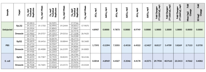
Table 2. qPCR calculations. Cq values of samples in three biological replicates (rep1, -2, -3), each in technical triplicates, obtained directly from the ViiA 7 Real-Time PCR system. Cq means (columns D, F, H) are determined as the mean of the three technical replicates of each biological replicate sample. From the Cq mean values, ΔCq values (columns I, K, M) and ΔΔCq values (columns J, L, N) are calculated for each biological replicate. ΔΔCq values are subsequently converted into fold changes (columns O, P, Q). For the final display of the data, the mean and SD of the data is determined, here presented in log2 scale (columns R, S). Please click here to view a larger version of this table.

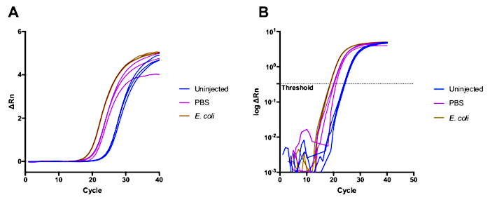
Figure 1. Fluorescent intensity represented as ΔRn. The value for ΔRn is obtained by subtracting the baseline fluorescence (Rn-) to the measured fluorescence (Rn+). In (A) ΔRn is plotted in a linear scale, while in (B) it is plotted using a log scale. The slashed line represents the threshold used to calculate the Cq of each sample. Please click here to view a larger version of this figure.

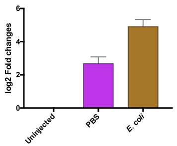
Figure 2. Changes in Drosocin RNA expression following injury and bacterial infection. Log2 transform of the fold RNA changes are shown. Flies injected with sterile PBS show a log2 fold increase of 2.7 in Drosocin expression, while flies infected with E. coli boost Drosocin expression by a log2 fold change of 4.9, compared to uninjected flies. Error bars represent the SD of the 3 biological replicates.

Applications and Summary

qPCR provides a quick and sensitive method to quantify nucleic acids among different samples. The protocol described here measures variation in RNA transcription levels due to different experimental conditions. qPCR has become the go-to technique when measuring the transcriptional output of a process, differences in gene dosage, or presence of (micro) organismal nucleic acids, relying only on primers that amplify the gene of interest. In contrast, detection of proteins is often limited to available antibodies or other specific tools. With its versatility and universal use, qPCR has had wide-reaching impacts on all areas of biological research and medicine.

References

Alberts, B., Johnson, A., Lewis, J., Morgan, D., Raff, M., Roberts, K., and Walter, P. (2014). Molecular Biology of the Cell, Sixth Edition (Garland Science).
Bustin, S.A., Benes, V., Garson, J.A., Hellemans, J., Huggett, J., Kubista, M., Mueller, R., Nolan, T., Pfaffl, M.W., Shipley, G.L., et al. (2009). The MIQE Guidelines: Minimum Information for Publication of Quantitative Real-Time PCR Experiments. Clinical Chemistry 55, 611–622.
Bustin, S., and Huggett, J. (2017). qPCR primer design revisited. Biomolecular Detection and Quantification 14, 19–28.
Kubista, M., Andrade, J.M., Bengtsson, M., Forootan, A., Jonák, J., Lind, K., Sindelka, R., Sjöback, R., Sjögreen, B., Strömbom, L., et al. (2006). The real-time polymerase chain reaction. Molecular Aspects of Medicine 27, 95–125.
Lemaitre, B., and Hoffmann, J. (2007). The host defense of Drosophila melanogaster. Annu. Rev. Immunol. 25, 697–743.
Ponton, F., Chapuis, M.-P., Pernice, M., Sword, G.A., and Simpson, S.J. (2011). Evaluation of potential reference genes for reverse transcription-qPCR studies of physiological responses in Drosophila melanogaster. Journal of Insect Physiology 57, 840–850.
Thornton, B., and Basu, C. (2011). Real‐time PCR (qPCR) primer design using free online software. Biochemistry and Molecular Biology Education 39, 145–154.
Tzou, P., Ohresser, S., Ferrandon, D., Capovilla, M., Reichhart, J.M., Lemaitre, B., Hoffmann, J.A., and Imler, J.L. (2000). Tissue-specific inducible expression of antimicrobial peptide genes in Drosophila surface epithelia. Immunity 13, 737–748.
Wittwer, C.T., Herrmann, M.G., Moss, A.A., 1997 Continuous fluorescence monitoring of rapid cycle DNA amplification.