Tracing de novo Lipids using Stable Isotope Labeling LC-TIMS-TOF MS/MS

Summary

Presented here is a method for screening lipid structures through stable isotope labeling by using their retention time, mobility, and fragmentation.

Abstract

Lipids are highly diverse, and small changes in lipid structures and composition can have profound effects on critical biological functions. Stable isotope labeling (SIL) offers several advantages for the study of lipid distribution, mobilization, and metabolism, as well as de novo lipid synthesis. The successful implementation of the SIL technique requires the removal of interferences from endogenous molecules. In the present work, we describe a high-throughput analytical protocol for the screening of SIL lipids from biological samples; examples will be shown of lipid de novo identification during mosquito ovary development. The use of complementary liquid chromatography trapped ion mobility spectrometry and mass spectrometry allows for the separation and lipids assignment from a single sample in a single scan (<1 h). The described approach takes advantage of recent developments in data-dependent acquisition and data-independent acquisition, using parallel accumulation in the mobility trap followed by sequential fragmentation and collision-induced dissociation. The measurement of SIL at the fatty acid chain level reveals changes in lipid dynamics during the ovary development of mosquitoes. The lipids de novo structures are confidently assigned based on their retention time, mobility, and fragmentation pattern.

Introduction

When analyzing lipid data, stable isotope labeling (SIL) is an effective method to assess metabolic pathways in living organisms. In this method, atoms within an analyte are replaced by stable isotopes containing ¹³C or ²H. These isotopes are further incorporated into precursors, which are later embedded within the fatty acids, labeling the areas in which they reside. With these isotopes, one is able to identify the distribution and metabolism of lipids, as they will contrast against the unlabeled background¹. Common mass spectrometry platforms are not able to distinguish the signal coming from endogenous molecules². The success of SIL requires the use of ultrahigh-resolution analytical tools. Liquid chromatography coupled to high-resolution trapped ion mobility spectrometry-parallel accumulation sequential fragmentation-time-of-flight tandem mass spectrometry (LC-TIMS-PASEF-TOF-MS/MS) allows the separation of labeled and nonlabelled species². The advantage of LC-TIMS-PASEF-TOF-MS/MS analysis is that the MS signal can be filtered by the retention time (RT) and mobility, thus reducing potential interferences of endogenous molecules, as well as quantification and separation of all desired species². In TIMS, an ion is first held stationary against a gas-mobile phase and subsequently released according to its mobility. This provides high-resolution mobilograms while operating at a lower voltage than earlier IMS instrumentation³. Mobilograms are plots of mass to charge versus drift time that can be used to distinguish between compounds based off of their drift time and amount of overlap⁴.

By using an additional PASEF technique, sequencing speed is greatly increased without sacrificing sensitivity⁵. The PASEF theory involves the accumulation of ions followed by their sequential release in the order of their mobility. This is done by accumulating ions in parallel alignment to their mobility. The accumulation in this fashion prevents ion loss. Furthermore, the precursor ion selection occurs simultaneously with the accumulation and release of the ions. With this method, PASEF selects multiple precursors in series during each TIMS scan, rather than the individual precursors per scan typical of a TIMS instrument that does not use PASEF. When the precursor ions are concurrently accumulated and released in 2 ms peaks within a TIMS scan of approximately 100 ms per frame, the signal is amplified by over one order of magnitude, therefore increasing the signal-to-noise ratio³. The PASEF addition to the TIMS increases the efficiency of the MS/MS. As the TIMS-PASEF is coupled with MS/MS, a more efficient fragmentation is possible. Unlike conventional MS/MS detection, the precursor signal is compressed from the TIMS-PASEF, and the fragment ions are detected simultaneously to the TIMS elution time and ion mobility position of the precursor³.

When acquiring data from a mass spectrometer, there are options in the scan mode desired. Data dependent acquisition (DDA) selects precursor ions from the MS1 scan based on their abundances, before fragmenting them and performing the MS2 scan. This scan mode fragments as many precursors as possible. The DDA approach is targeted, and results will depend on the ion selection³. However, DDA-PASEF often has problems in the reproducibility between replicates. While DDA is a great tool in a focused analysis, complex mixtures have greater difficulty in their data acquisition⁶. This is because only a small amount of ions can be monitored simultaneously³. Data independent acquisition (DIA) is a method where preselected windows of m/z are fragmented independently from their intensity, and all are scanned within the range⁷. With this scan mode, entire ion clouds are transmitted from the IMS to the mass spectrometer³. In proteomics studies this results in greater amounts of proteins being quantified in a shorter time span compared to DDA. In addition, DIA misses fewer m/z values compared to DDA. Therefore, this alternative has shown great improvements in data reproducibility in signal to noise ratio and better quantification than DDA. In this present work, our goal is to implement DIA to the method reported by Tose et al.². We improved the reproducibility and intensity of signals, yielding further and more conclusive information on SIL lipids mobilization, distribution and metabolism in biological samples taking advantage of DDA and DIA acquisition.

Protocol

1. Sample preparation

1. Insect dissection
   1. Dissect Aedes aegypti mosquito ovaries when they are 7-days old in a phosphate buffered saline solution using microneedles.
   2. Collect eight ovaries from phosphate buffered saline solution using microneedles and store in 1.5 mL microcentrifuge tubes at -80 ˚C.
   3. Collect ovaries in biological replicates.
2. Lipid extraction
   1. Add 10 µL of internal standard (ISTD) into the eight collected ovaries in a concentration of 1 ppm. The ISTD is a labeled lipid mixture with seven deuterium of 1-pentadecanoyl-2-oleoyl-sn-glycero-3-phosphocholine-D7 (15:0-18:1 (D7) PC), lysophosphatidylcholine-D7 (18:1 (D7) Lyso PC), 1-pentadecanoyl-2-octadecenoyl-glycero-3-phosphoethanolamine-D7 (15:0-18:1 (D7) PE), 1-oleoyl-2-hydroxy-sn-glycero-3-phosphoethanolamine-D7 (18:1 (D7) Lyso PE), 1-pentadecanoyl-2-oleoyl-sn-glycero-3-phosphoinositol-D7 (15:0-18:1 (D7) PI), 1-pentadecanoyl-2-oleoyl-sn-glycero-3-phospho-L-serine-D7 (15:0-18:1 (D7) PS), 1,2-dipentadecanoyl-3-octadecenoyl-sn-glycerol (15:0-18:1-15:0 (D7) TAG), 1-pentadecanoyl-2-octadecenoyl)-sn-glycerol-D7 (15:0-18:1 (D7) DAG), 2-octadecenoyl-sn-glycerol-D7 (18:1 MAG (D7)), cholesteryl oleate-D7 (18:1 (D7) Chol Ester).
   2. Wait until dry at room temperature. Add 100 µL of butanol/methanol and 3 µL of butylated hydroxytoluene. Homogenize manually for 10 s with 1.5 mL polypropylene pestles.
   3. Rinse the pestle with 200 µL of butanol/methanol and combine with the homogenized solution.
   4. Sonicate the microcentrifuge tube at room temperature and medium power for 30 min.
   5. Centrifuge tubes at 1600 x g for 10 min at 20 °C. Transfer the supernatant into autosampler vial with 300 µL of silanized glass inserts.

2. Instrument setup

1. Preparing the mobile phase
   1. Prepare mobile phase with a composition of 30:40:30 (mobile phase A) and 10:5:85 (mobile phase B) using acetonitrile, water, and isopropanol as the respective proportion. In both mobile phases, add 10 mmol/L ammonium formate in water and 0.1% formic acid to create a buffer condition.
   2. Weigh out 3.15 g of ammonium formate in 10 mL of water. Add 500 µL of this solution in 12.5 mL of water. In sequence, put into a 250 mL volumetric flask and fill with isopropanol to about 2/3 of the flask. Mix by swirling.
   3. Add 250 µL of formic acid (85%), fill with 25 mL of acetonitrile and isopropanol to the fill line of 250 mL, and mix.
2. In the MS system, on the left side of the screen at MS settings, determine the mass range by selecting 50 as the minimum and 1850 as the maximum scan setting.
   1. Select Polarity as positive ion mode. Select the scan mode as DIA-PASEF. To do this, select Tune and open analysis method from a previous DDA method with the following LC parameters.
      1. For gradient separation:
         Sample injection: 0% B, hold time 1 min.
         Increase to 55% B, hold until 6.4 min.
         Increase to 65% B, hold until 24 min.
         Increase to 88% B, hold until 40.8 min.
         Increase to 95% B, hold until 48.1 min.
         Decrease to 35% B, hold until 56 min.
         Decrease to 0% B, hold until 60 min.
      2. For HPLC conditions:
         Injection volume: 5 µL
         Solvent rate: 0.25 mL/min
         ​Total run time: 60 min, in which 5 min are to precondition the column.
      3. Prepare the liquid chromatograph by inserting the column into the liquid chromatograph. Run a blank to clean the column and test for leaks. This can be seen in the instrument not holding pressure or flow.
3. To create a new method, perform the steps described below (Figure 1 and Figure 2).
   1. Open the software and click on Connect all instruments. If the connection is successful, the LC system will beep once, and the control screen lists HyStar in the Status box without any error messages.
   2. Click on the Acquisition tab. On the Sample Table Navigator, find the tag dropdown menu and select a previous method.
   3. Double the latest sample table. Click on Save As… and save new sample list with the format: YYYYMMDD_LIP_C30_(XXXX) where (XXXX) is a short descriptor of the analysis.
   4. Right click on the separation method and click on Edit Method. Click on Edit Module Method.
   5. Click on Download. If successful, Download succeeded will pop up. Close screen without saving method.
   6. Under MS settings go to TIMS settings, select the 1/k0 start at 0.70 and 1/k0 end at 1.85. Set the ramp time to 150 ms. With this, the duty cycle and ramp rate are automatically adjusted.
   7. At the bottom window select the Source tab. Select the source type as ESI and set the end plate offset to 800 V and the capillary to 4500 V. Check the nebulizer box and set the pressure to 4.0 bar. Set the dry gas to 4.0 L/min and the dry temperature to 250 °C.
   8. To the right of the source tab, select the Tune tab. Click the General Sub tab and under the transfer heading ensure the following parameters:
      Deflection 1 delta: 70 V
      Funnel 1 RF: 250 vpp
      isCID energy: 0 eV
      Funnel 2 RF: 250 vpp
      ​Multipole RF: 500 vpp.
      1. Under the collision cell heading ensure the following parameters:
         Collision energy: 6.0 eV
         Collision RF: 1200 vpp.
      2. Under the quadrupole heading ensure the following parameters:
         Ion energy: 6 eV
         Low mass: 250 m/z.
      3. Under focus pre-TOF tab ensure the following parameters:
         Transfer time: 45 µs
         ​Pre-pulse storage: 5.0 µs.
   9. Click the Processing Sub tab. Under mass spectra peak detection ensure the following parameters:
      Absolute threshold: 667
      ​Absolute threshold (per 100 ms AccuTime): 445.
      1. Under mobility peak detection ensure the following parameters:
         ​Absolute threshold: 30.00.
   10. Click the TIMS subtab. Under the offsets tab ensure the following parameters:
       Δt1: -20 V
       Δt2: -150 V
       Δt3: 70 V
       Δt4: 150 V
       Δt5: 0 V
       Δt6: 150 V
       ​Collision cell: 300 V.
   11. To the right of the tune tab, click the MS/MS tab. Under the precursor ions tab ensure the following parameters:
       Number of PASEF ramps: 8
       Charge minimum: 1
       ​Charge maximum:1.
       1. Under the scheduling tab, click Advanced and ensure the following parameters:
          Intensities: 0,1500, 5000, 10000
          Repetition: 1, 10, 5, 1
          Intensity Threshold: 1500.
       2. Under the active exclusion tab ensure the following parameters:
          Active exclusion check mark
          ​Release after: 0.4 min.
       3. Under collision energy settings ensure the following parameters:
          K0 (V-s/cm³): 0.70, 1.60
          ​Collision energy (eV): 20.00, 35.00.
       4. Under isolation width settings ensure the following parameters:
          Mass (m/z): 622, 1222
          Width (m/z): 1.00 2.50.
   12. DIA -PASEF set up: Select DIA-PASEF from the MS settings scan mode on the left. Under the MS/MS tab, select Window Editor. Here, ensure the following parameters (Figure 3):
       Window settings: Mass width: 50 Da; Mass overlap: 0.0 Da; Calculate from polygon: mass steps; Number of mobility windows: 1.

3. Calibration

1. Instrument calibration (Figure 4)
   1. Under the Calibration sub tab click on m/z, select Tuning Mix from the drop box and click Calibrate at the bottom right corner.
   2. Continue to click Calibrate until a score of 100% is achieved.
   3. Now select the Mobility tab and follow the same steps as above until the 100% calibration score is reached.
2. Calibration curve
   1. Spike lipid internal standard mixture with 10 µL of deuterated internal standard mixture.
      Use seven calibration points from 0.1-500 ng/mL of standard mixture with 10 µL of the deuterated internal standard mixture.
   2. Manually annotate the fatty acid chains based of the PASEF MS/MS patterns already described in².
3. SIL labeling efficiency
   1. Calculate the ratio of the area of the SIL containing isotopes to the area of the non-SIL containing isotopes.
   2. Calculate the theoretical patten by determining the probability of finding a labeled atom any site.
   3. Calculate SIL enrichment by fitting the experimental isotope profiles with the theoretical pattern simulated on data analysis software.
4. Starting the run
   1. Activate column oven by clicking the Thermometer button. Activate pumps by clicking the Valve button.
   2. Set MS method to the method saved earlier. Verify that injection volume is 5 µL and that line 1 will target vial 20:1.
   3. Ensure that vial 20:1 has 50% IPA/ACN. Save sample list.
   4. Start sequence and verify that a successful injection is made (confirmed by a message displayed on the system stating injected).
   5. Copy line 1 and paste below to generate a new line. Populate line 2 with samples depending on current experiment. Make sure that the correct position in the autosampler is used.
   6. If mobile phase is fresh, perform peak shape test first by injecting the lipid mixture standards from the manufacturer. Compare with previous results.² The standards are a lipid mixture of 1-pentadecanoyl-2-oleoyl-sn-glycero-3-phosphocholine (15:0-18:1 PC), lysophosphatidylcholine (18:1 Lyso PC), 1-pentadecanoyl-2-octadecenoyl-glycero-3-phosphoethanolamine (15:0-18:1 PE), 1-oleoyl-2-hydroxy-sn-glycero-3-phosphoethanolamine (18:1 Lyso PE), 1-pentadecanoyl-2-oleoyl-sn-glycero-3-phosphoinositol (15:0-18:1 PI), 1-pentadecanoyl-2-oleoyl-sn-glycero-3-phospho-L-serine (15:0-18:1 PS), 1,2-dipentadecanoyl-3-octadecenoyl-sn-glycerol (15:0-18:1-15:0 TAG), 1-pentadecanoyl-2-octadecenoyl)-sn-glycerol (15:0-18:1 DAG), 2-octadecenoyl-sn-glycerol (18:1 MAG), cholesteryl oleate (18:1 Chol Ester).
   7. Make sure new lines have the correct separation method and not the preconditioning method used in line 1. Make sure that the MS method is correct (current day's method).
   8. Check that the correct processing method is loaded and that the Run Automated Process is enabled.
   9. Save sample list to make sure that samples are analyzed after the current run finishes.

4. Data analysis

1. Open Data Analysis software (Figure 5). At the top left corner click on the File button and Select Open…
2. Select the files of choice. Right click on the file name and select Properties.
   1. Select Calibration Status (Figure 6). At the drop-down box, select Initial Calibration for the mass spectrometer. Ensure that all errors are less than 1 ppm.
   2. Next, select Initial Mobility Calibration and confirm that the error is less than 1 ppm.
   3. Right click on Chromatogram and select Edit Chromatogram (Figure 6C). At Type, click the drop-down box and select Extracted Ion Chromatogram (Figure 6D). Under filter, select All MS and with scan mode select All. This is to view the peaks for the molecule of interest rather than only its fragments.
      1. Below this, there are two filter options for molecule selection: Masses or Formula. If Masses is selected, one can choose the theoretical m/z of the molecules of interest. For this case select 829.7985 m/z. If Formula is selected, one can choose the formula for the molecule as well as the ion forms of interest for the chromatogram. In this case, select ammonium [M+NH₄]. This is due to the ammonium buffer in the mobile phase that will favor ionization in this ion form (Figure 7).
      2. For width select ±1. For polarity ensure that it maintains positive mode. Under Mobility select 1.455-1.465. This is done to filter out any molecules that do not fall within these values and isolate the molecule of interest.
3. Once parameters selected, click Add > OK at the top right. After a short amount of time, the software will process the selections and output a chromatogram.
4. Right click at the baseline at the start of the peak of interest and drag while holding to the end of the peak. This manual integration will provide a live mass spectrum of fragments within that retention time.
5. Mobilogram
   1. Right click at the left of the screen on Mobilogram and select Edit Mobilogram (Figure 8). A window named Edit Mobilogram Traces will appear. Follow the same steps C.e.i.1 to C.e.i.5 (Figure 9).
   2. At Retention Time input the retention time of the peak of interest. In this case, 37.45-37.55 min.
   3. Once parameters selected, click Add > OK at the top right. After a short amount of time, the software will process the selections and output a chromatogram.
6. For extracted ions, repeat steps 4.2.3.1-4.3.2.2 until a list of ions is formed.
7. At the bottom of the MS window, select Profile MS and Fragment MS. This will allow a spectrum view of ions from full scan and PASEF.
   1. At spectrum view, right click and select Copy Compound Spectra. With the spectrum data that appears at the right, one can find more information on one's compound such as resolution resolving power, intensity, and signal to noise ratio (S/N; Figure 10).
8. Processing
   1. To process the data, manually integrate the chromatogram and mobility peaks to yield valuable information on the molecule of interest (Figure 10).
   2. Right click Find and select Integrate Only chromatogram or mobilogram (Figure 11). Left click and highlight the desired peak. This information includes retention time, area, S/N, and mobility.

Representative Results

The stable isotope labeling facilitates the visualization of triglycerides in lipid dynamics studies of female mosquito ovaries. In the 2D mobility domain, the triglyceride 48:1 is displayed in a region with a specific retention time in relation to mobility 1/K₀. The intensity of the triglyceride can be visualized by a darker blue line. Other spots represent additional triglycerides found within the ovary. The retention times and mobilities vary due to the differences in masses and structures, therefore appearing in different areas of the graph. These differences are key when distinguishing between triglycerides in a sample (Figure 12A,B). The amplified mass spectrum projection of the region displays a 48:1 triglyceride ion coupled to an ammonium ion at 822 m/z. Other triglycerides, such as 50:2 and 52:3, are also visualized, but at higher m/z regions due to the differences in structure, size, and fragmentation (Figure 12C,D). In this example, we were interested in analyzing the deuterium labelled isotopes. The region for TG 48:1 was further amplified to visualize the isotopically labeled ions. As the amount of deuterium on the ion increases, the intensity of the peak decreases. This happens as there are lower occurrences of the high deuterium labeled ions. The m/z ratio increases slightly with each addition of deuterium due to mass increases. These intensities will further determine the amount of each isotope present within the sample.

When assessing the intensities of the fragments in the mass spectrum, one must compare the non-labeled isotopes with those labeled with ²H (Figure 12E). In blue is the non-labeled intensity with the dashed black lines as theoretical intensities. In red, the isotope labeled results are observed. They display greater intensities than both the non-labeled and theoretical intensities. The enrichment of the species with isotopic labeling yields a greater intensity than the non-labeled theoretical species. The greater intensities allow visualizing the triglycerides due to the district discrepancies. The fragmentation also plays a key role in the identification of lipids, as the PASEF will provide increased fragmentation compared with the full scan MS/MS. This is because the fatty acids in the lipid chains may fragment in different patterns, therefore the lines in the spectra show the intensity of the fragments based on the fragmentation process of the triglyceride (Figure 12F). This provides structural information on the fatty acid and helps to establish which isomer of a species is present. When analyzing data from the DIA method, the number of fragments will increase, therefore resulting in a better MS/MS scan and superior identification than in a typical DDA method.

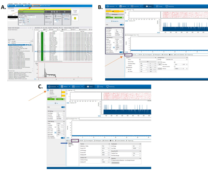
Figure 1: Typical home screen of the software. The home screen allows for method creation and starting the instrument. (A) Software screen containing TIMS and MS/MS control settings. At the bottom of the screen is the source tab to edit those controls on the instrument. (B) Software screen with the tune tab opened. (C) Here, one can prepare the instrument for general tune. Please click here to view a larger version of this figure.

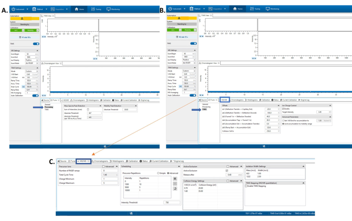
Figure 2: Software screen with the tune tab opened. Here one can edit the processing tune parameters. (A) Software screen with the tune tab opened. Here one can edit the tune parameters for the TIMS portion of the instrument. (B) Software screen with the MS/MS tab selected at the bottom of the screen. (C) Here one can edit parameters for the tandem mass spectrometer. Please click here to view a larger version of this figure.

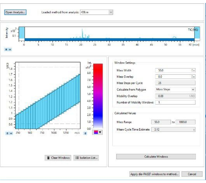
Figure 3: Screen for selecting DIA-PASEF window widths. Here one can edit the colors for abundance as well as edit the size of the windows for data acquisition. Please click here to view a larger version of this figure.

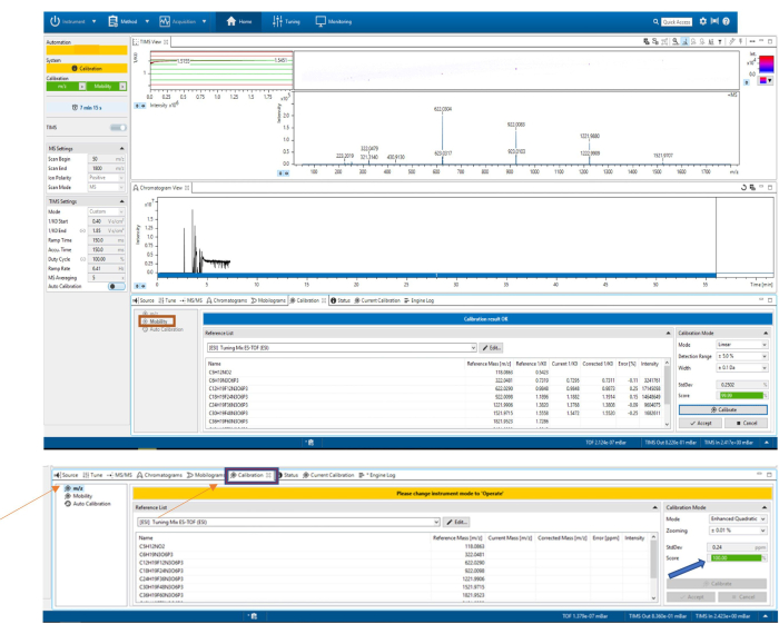
Figure 4: Calibration of the mass spectrometer by mass to charge ratio (m/z). The reference list is selected for the calibration. (A) At the bottom right, the Calibrate button is clicked until an acceptable value appears. Calibration of the ion mobility spectrometer by mobility. The reference list is selected for the calibration. (B) At the bottom right, the Calibrate button is clicked until an acceptable value appears. Please click here to view a larger version of this figure.

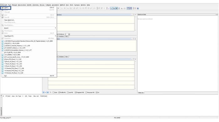
Figure 5: Typical home screen for the data analysis software. To open a file, the top left File button is clicked for the drop box with options to appear. Please click here to view a larger version of this figure.

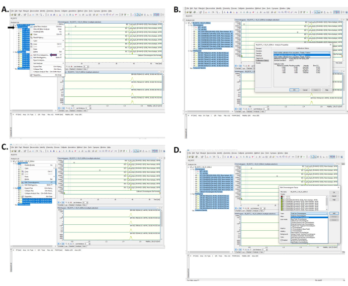
Figure 6: Data analysis software. The software screen confirming a successful calibration with (A) how to select calibration results and (B) selecting the calibration category. (C) Selecting a chromatogram to analyze and (D) selecting an extracted ion chromatogram. Please click here to view a larger version of this figure.

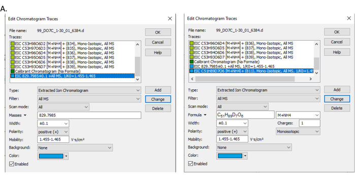
Figure 7: Pop-up screen. Pop-up for selecting and extracting ion chromatogram by (A) mass filter and (B) formula filter. Please click here to view a larger version of this figure.

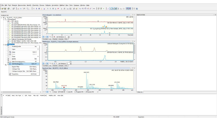
Figure 8: Data Analysis software. The software screen where at the left, a mobilogram is selected for analysis. Please click here to view a larger version of this figure.

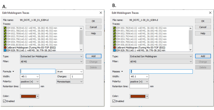
Figure 9: Pop-up screen for mobilogram. Pop-up for selecting an extracted ion mobilogram by (A) mass filter and (B) formula filter. Please click here to view a larger version of this figure.

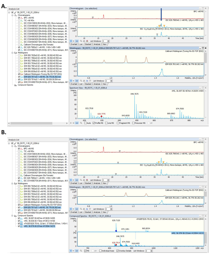
Figure 10: Data analysis screen. (A) The software screen; highlighted on the left one can form an extracted ion list. (B) Data analysis screen where at the bottom a compound spectrum from the extracted ions is prepared. Please click here to view a larger version of this figure.

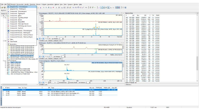
Figure 11: Data analysis screen. The software screen demonstrating the results of a manual integration of compound spectra. Please click here to view a larger version of this figure.

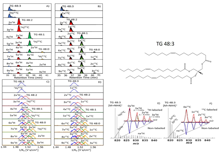
Figure 12: LC-TIMS MS Result. (A) The LC-TIMS MS at 4 days after feeding ²H-labelled sucrose diet and the insect ovaries can be seen in the 2D mobility domain. (B) Typical MS projections for the signal corresponding to TG 48:1, TG 50:2 and TG 52:3 from labelled sample. (C) Amplified MS region 822 – 827 m/z denoting labelled TGs profile. (D) Pay particular attention to MS peaks in red are amplified the isotope profile. (E-F) The ²H labelled isotope profile is highlighted in red; below non-labelled isotope profile are highlighted in blue. The theoretical isotope profiles are indicated as dash lines (¹³C in black; ²H in green). A potential structure for triglyceride 48:3 is also displayed on the top right. Please click here to view a larger version of this figure.

Discussion

When assessing the use of this protocol, it is essential to ensure the DIA-PASEF and MS/MS parameters are applicable to the triglycerides in question. Specifically, mobility windows and window width should follow the pattern of the triglycerides. This can be determined with a previous run using the DDA method. When tracking the triglycerides in the internal standard, the windows for the DIA set up should cover all the pre-identified molecules of interest. The windows should all be of equal sizes, and the ranges fall within the m/z and 1/k0 of the desired compounds (Figure 7). With an incorrect sizing of the windows, the ions to be fragmented will be skipped over and the yield spectra would have lower reproducibility. Essentially, without proper optimization of a window range in lipidomics, DIA results will not enhance the DDA data. The windows should represent a stepwise shape for the data acquisition process. If this is not the case, the parameters amongst the DIA-PASEF window set up should be altered to be representative of the complete lipid profile. Without this step, critical fatty acids will be omitted from the data acquired.

Instrumental limitations include mostly those that come with LC-MS methods. This includes multiplexing limitations in peak width. Therefore, there must be an optimization in peak elution for an appropriate quantitation, promoting selectivity during the data acquisition. Typically, this is with selected precursors such as with DDA. However, with DIA, no precursors are selected, therefore risking limitations in instrumental selectivity⁸. While DIA methods provide increased fragmentation, there are still limitations present. The most prominent limitation is the reduction in precursor selectivity. The windows for a DIA method are 5 to 10 times wider than a typical DDA method. Consequently, while allowing for greater fragmentation, it could reduce duty cycle and serial acquisition. This can be observed in mass spectrometers that use a stepped quadrupole. As there is no selection of precursors and which ions should be fragmented, static isolation windows are sequentially cycled through to cover the m/z window. As the window is much greater than a typical DDA method, one must use wider ranges to attempt to gain sensitivity⁹. The issue in the serial acquisition therefore reduces the sensitivity. A second limitation involves library generation. It is time consuming and requires extensive amounts of samples to formulate. While external libraries can be used, the fragmentation patterns may differ between experimental conditions and instrumentation¹⁰.

When analyzing lipid data using stable isotope labeling, it is necessary to minimize interference from other molecules found in the organism. This is done by using high resolution analysis tools such as the LC-TIMS-TOF-MS/MS². Currently, the use of these high-resolution tools to separate the labeled isotopes from the background noise is still very novel compared to traditional methods. Traditional instrumental considerations implement separation by gas chromatography followed by chemical or electron ionization. This allows for either chemical derivation with pentafluorobenzyl bromide or fragmentation from electron ionization. It is more recently where LC-MS is employed in isotopic studies. Use of high-resolution mass spectrometers allows for high mass accuracy and the ability to conduct multi-tracer studied by using multiple isotopic labels rather than a single isotope. Without the high resolution of the instrument one would be unable to differentiate between different labeling degrees such as ¹³C₂ and ¹³C. This allows for increased information from a single run compared to traditional instrumentation with lower resolution¹⁰.

While DIA has better reproducibility than DDA, other emerging data acquisition methods can compare. Hybrid DIA-DDA strategies such as p-SMART are able to combine the strengths of each method to maintain great detection and quantitation, while keeping the high level of targeted qualitative analyses. In this method, using one matched product ion can increase the DIA sensitivity and selectivity, as it will narrow the DIA windows in comparison to a wide untargeted approach⁸. In lipidomics, the structure of a triglyceride can vary with the isomeric structure. PASEF allows for the visualization of various fragmentation patterns, improving species identification². With the use of DIA-PASEF, the increased fragmentation provides information on isomers as many fragments similarly to others, which are normally unable to be resolved due to the limitations of the DDA method. This information provides evidence on what fatty acids are present in the mosquito ovaries. This method can be applied to other de novo lipids studies in diverse organisms.

Materials

Accucore C30 colum	Thermo Fisher Scientific	27826-252130
Bruker Compass Data Analysis	Bruker Daltonics Inc	2363525870	Version 5.2
d-Glucose-13C6	Sigma-Aldrich	389374
eppendorf tubes	Fisher Scientific	14-282-300
EquiSplash Lipidomix	Avanti Polar Lipids	330731-1EA
glass vials	Thermo Fisher Scientific	11-417-236
heavy water (2H2O)	Sigma-Aldrich	1.13366
polypropylene pestles	Fisher Scientific	BAF199230001
Prominence LC-20 CE ultrafast liquid chromatograph	Shimadzu	L20234651907
silanized glass inserts	Thermo Fisher Scientific	03-251-826
Sucrose-13C12	Sigma-Aldrich	605417
timsTOF	Bruker Daltonics Inc	1.84443E+11
Tuning Mix Calibration Standard	Agilent Technologies	36

References

1. Stokvis, E., Rosing, H., Beijnen, J. H. Stable isotopically labeled internal standards in quantitative bioanalysis using liquid chromatography/mass spectrometry: Necessity or not. Rapid Commun Mass Spectrom. 19 (3), 401-407 (2005).
2. Tose, L. V., et al. Coupling stable isotope labeling and liquid chromatography-trapped ion mobility spectrometry-time-of-flight-tandem mass spectrometry for de novo mosquito ovarian lipid studies. Anal Chem. 94 (16), 6139-6145 (2022).
3. Meier, F., Park, M. A., Mann, M. Trapped ion mobility spectrometry and parallel accumulation-serial fragmentation in proteomics. Mol Cell Proteomics. 20, 100138 (2021).
4. Basit, A., Pontis, S., Piomelli, D., Armirotti, A. Ion mobility mass spectrometry enhances low-abundance species detection in untargeted lipidomics. Metabolomics. 12 (3), 50 (2016).
5. Meier, F., et al. Online parallel accumulation-serial fragmentation (PASEF) with a novel trapped ion mobility mass spectrometer. Mol Cell Proteomics. 17 (12), 2534-2545 (2018).
6. Koopmans, F., Ho, J. T. C., Smit, A. B., Li, K. W. Comparative analyses of data independent acquisition mass spectrometric approaches: DIA, WiSIM-DIA, and untargeted DIA. Proteomics. 18 (1), 1700304 (2018).
7. Fernández-Costa, C., et al. Impact of the identification strategy on the reproducibility of the DDA and DIA results. J Proteome Res. 19 (8), 3153-3161 (2020).
8. Prakash, A., et al. Hybrid data acquisition and processing strategies with increased throughput and selectivity: PSMART analysis for global qualitative and quantitative analysis. J Proteome Res. 13 (12), 5415-5430 (2014).
9. Tsou, C. C., et al. DIA-umpire: Comprehensive computational framework for data-independent acquisition proteomics. Nat Methods. 12 (3), 258-264 (2015).
10. Triebl, A., Wenk, M. R. Analytical considerations of stable isotope labelling in lipidomics. Biomolecules. 8 (4), 151 (2018).
Tags
check_url/65590?article_type=t
Play Video
Cite This Article
Castro, K. D., Tose, L. V., Willetts, M., Park, M. A., Nouzova, M., Noriega, F. G., Fernandez-Lima, F. Tracing de novo Lipids using Stable Isotope Labeling LC-TIMS-TOF MS/MS. J. Vis. Exp. (210), e65590, doi:10.3791/65590 (2024).