JoVE Science Education
General Chemistry
A subscription to JoVE is required to view this content.  Sign in or start your free trial.
JoVE Science Education General Chemistry
Spectrophotometric Determination of an Equilibrium Constant
  • 00:00Overview
  • 01:02Principles of the Equilibrium Constant
  • 03:08Creating a Calibration Curve for Fe(SCN)2+
  • 04:38Measuring K for the Fe(SCN)2+ System
  • 05:28Results
  • 06:59Applications
  • 08:33Summary

평형 상수의 분광측정 결정

English

Share

Overview

출처: 마이클 에반스 박사 연구소 — 조지아 공과대학

평형상시, K,화학시스템에 대한 제품 농도의 비율은 평형에서 반응성 농도에 대한 비율이며, 각각 각각 각 스토이치오메트릭 계수의 힘으로 상승한다. K의 측정은 화학 적 평형시스템에 대한 이러한 농도의 결정을 포함한다.

단일 컬러 성분을 포함하는 반응 시스템은 분광계로 연구될 수 있다. 착색 성분에 대한 흡광도와 농도 사이의 관계는 반응 시스템에서 의 농도를 결정하는 데 사용됩니다. 무색 성분의 농도는 균형 잡힌 화학 방정식과 착색 성분의 측정 된 농도를 사용하여 간접적으로 계산될 수 있습니다.

이 비디오에서 Fe(SCN)2+에 대한 맥주의 법칙 곡선은 경험적으로 결정되고 다음 반응을 위해 K 측정에 적용됩니다.

Equation 1

반응제의 다른 초기 농도를 가진 4개의 반응 시스템은 K가 초기 농도에 관계없이 일정하게 남아 있다는 것을 보여주기 위하여 조사됩니다.

Principles

Procedure

1. Fe (SCN)2 + 맥주의 법칙 곡선 결정 증류수를 빈물로 사용하여 보이는 분광광계를 교정합니다. 시험관에 1.0mL × 10-4 M Fe(NO3)3용액을 추가합니다. 동일한 테스트 튜브에 0.50 M KSCN 솔루션의 5.0 mL을 추가합니다. 동일한 테스트 튜브에 0.10 M HNO3 솔루션의 4.0 mL을 추가합니다. 장갑을 낀 손가락으로 튜브를 덮고 부드럽게 흔들어 섞습?…

Results

Table 4 lists the absorbance and concentration data for solutions 1 – 5. Concentrations of Fe(SCN)2+ were determined from initial concentrations of Fe3+ under the assumption that all of the Fe3+ is converted to Fe(SCN)2+. A large excess of SCN was used in tubes 1 – 5 to ensure that this assumption holds true.

The molarity [Fe(SCN)2+] and absorbance are plotted in Figure 2. The measured absorbances agree well with Beer's law.

Table 5 lists measured absorbances and calculated K values for tubes 6 – 9. K values were determined using the ICE table method. Initial reactant concentrations were based on the known molarities of Fe3+ and SCN in the reactant solutions and the total volume of the reaction (10 mL). The equilibrium concentration of Fe(SCN)2+ was determined by dividing measured absorbance by the molar absorptivity of Fe(SCN)2+. Because all of the product was formed from the 1:1 reaction of Fe3+ and SCN, the equilibrium concentration of Fe(SCN)2+ corresponds to the decrease in concentration of the reactants. Table 6 shows the process for test tube 6.

The equilibrium constant is calculated from the concentrations in the equilibrium row. For test tube 6,

Equation 6

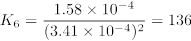
The mean K value was 147 ± 11, illustrating that K is roughly constant over the range of concentrations studied.

Figure 2
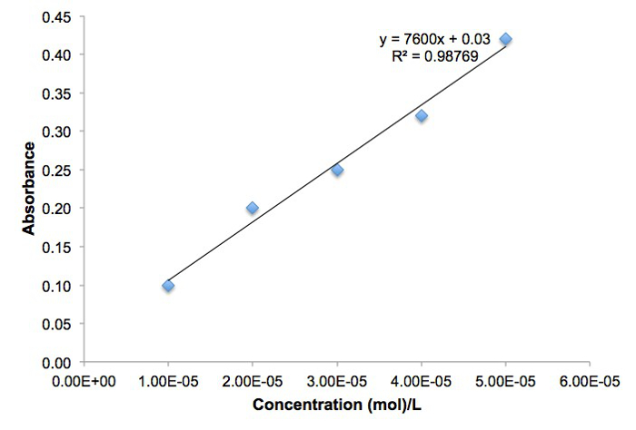
Figure 2. Line graph of Absorbance versus Concentration for Fe(SCN)2+.

Tube [Fe(SCN)2+] (mol/L) Absorbance
1 1.00 x 10⁻⁵ 0.10
2 2.00 x 10⁻⁵ 0.20
3 3.00 x 10⁻⁵ 0.25
4 4.00 x 10⁻⁵ 0.32
5 5.00 x 10⁻⁵ 0.42

Table 4. Absorbance versus Concentration Data for Fe(SCN)2+.

Tube Absorbance K
6 0.120 136
7 0.268 161
8 0.461 142
9 0.695 150

Table 5. Measured absorbance values and calculated K for the reaction of iron (III) with thiocyanate.

[Fe3+] (mol/L) [SCN] (mol/L) [Fe(SCN)2+] (mol/L)
Initial 3.57 x 10⁻⁴ 3.57 x 10⁻⁴ 0
Change –1.58 x 10⁻⁵ –1.58 x 10⁻⁵ +1.58 x 10⁻⁵
Equilibrium 3.41 x 10⁻⁴ 3.41 x 10⁻⁴ 1.58 x 10⁻⁵

Table 6. The ICE table that illustrates the process used for test tube 6.

Applications and Summary

The equilibrium constant provides useful information about the extent to which a reaction will proceed to form products over time. Reactions with a large value of K, much larger than 1, will form products nearly complete given enough time (Figure 3). Reactions with a value of K less than 1 will not proceed forward to a significant degree. The equilibrium constant thus serves as a measure of the feasibility of a chemical reaction.

Figure 3
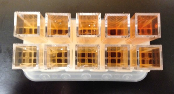
Figure 3. The equilibrium constant of this reaction is greater than 1. A significant amount of colored product forms in each case, even though the initial concentrations of reactants differ.

The equilibrium constant also provides useful thermodynamic information about the changes in free energy, enthalpy, and entropy in the course of a chemical reaction. The equilibrium constant is related to the free energy change of reaction:

Equation 7

The free energy change of reaction is in turn related to the enthalpy and entropy changes of reaction:

Equation 8

Measurements of the temperature dependence of K can reveal the enthalpy change ΔH and the entropy change ΔS for a reaction. In addition to providing chemists with insight into patterns in molecular behavior, tables of thermodynamic data can be used to identify reactions with favorable thermodynamic properties. For example, redox reactions that release large amounts of energy (associated with negative ΔG values) are attractive candidates for batteries.

Values of K for acid dissociation reactions (Ka values) are useful for predicting the outcomes of acid-base reactions, which are thermodynamically controlled. Strong acids are associated with large Ka values and weak acids with small Ka values. pH indicators are weak acids with differently colored acidic and basic forms, and the pKa (the negative base-10 logarithm of Ka) of an indicator represents the pH at which a color change occurs as an acid or base is added to a solution of the indicator.

Similarly, Ka values are used in the preparation of buffer solutions to achieve a target pH value. The pKa of a weak acid represents the pH at which the acid and its conjugate base are present in the solution in equal concentrations. When equal amounts of a weak acid and its conjugate base are dissolved in a solution, the pH of the solution equals the pKa of the weak acid.

Transcript

Determining the equilibrium constant of a chemical reaction can provide important information about the extent to which it will form products over time.

Every chemical reaction is associated with an equilibrium constant, K, which reflects the ratio of the concentrations of the products and reactants when the reaction has stopped progressing. To measure K, these concentrations must be determined.

If a reaction contains a single colored component, its interaction with light can be measured to discern its concentration. The concentrations of the uncolored components can then be calculated indirectly using the balanced chemical equation. This video will illustrate the use of a spectrophotometer to empirically determine the equilibrium constant for an iron thiocyanante reaction.

Most chemical reactions proceed in both forward and reverse directions. As the reaction progresses, it reaches a point where the forward and reverse reactions occur at the same rate. This is known as chemical equilibrium. At this steady state, the ratio of product concentrations to reactant concentrations, each raised to the power of their stoichiometric coefficients, corresponds to the equilibrium constant, K. To measure K for a system of interest, the coefficients should be known, and the concentrations must be determined, either directly or indirectly. According to the Beer-Lambert law, the concentration of a colored species is proportional to its absorbance, which is the amount of energy it absorbs at a specific wavelength of light. This can be expressed mathematically, where A is absorbance, epsilon is the molar attenuation coefficient, which is compound-specific, l is the path length through the sample, and c is concentration. A calibration curve is created by testing multiple solutions of known concentration, and plotting the resulting absorbance values. With this calibration curve, solutions of unknown concentration can be studied. Absorbance measurements are used to determine the concentration of the colored species. Then, the concentrations of the remaining reactants and products can be calculated. The following procedure will study the reaction of iron three with thiocyanate to form an iron thiocyanate complex.

Once the concentrations have been determined, the value for K can be calculated with an Initial-Change-Equilibrium, or ICE, table which will be explained further in the results.

Now that you understand how spectrophotometric methods can be used to determine the equilibrium constant, you are ready to begin the procedure.

Before measuring the sample, a calibration curve must be generated.

To begin, zero a UV-vis spectrophotometer using distilled water as a blank to represent no absorbance. When inserting a cuvette into the spectrophotometer, ensure that it is oriented so light passes through the transparent sides, and that the liquid level is above the path of the beam.

Then, prepare 5 test tubes containing the indicated volumes of each reactant solution as shown in the text protocol, which will yield varying concentrations of the product. Cover each tube with a gloved finger, and gently shake to mix. Allow the tubes to rest for 10 min.

Use a Pasteur pipette to transfer a small quantity of the mid-concentration sample, solution 3, to a cuvette, and place it in the spectrophotometer. Acquire a spectrum and record the λmax (maximum wavelength), lambda max, and its absorbance. Then, beginning with the most dilute solution, measure the absorbance of all remaining solutions at the λmax (lambda max). Use the same cuvette for all measurements, making sure to rinse 3 times in between each sample. Repeat this process for solutions 2 – 5.

Plot the measured absorbance versus concentration of iron thiocyanate for each solution. Determine the line of best fit for the data. The slope of this line is the molar attenuation coefficient.

Now that the data for the standard solutions has been acquired, prepare four medium test tubes containing the indicated volumes of solutions as shown in the text protocol.

Cover each tube with a finger and gently shake to mix. Allow them to stand for at least 10 min. This resting period allows the solutions to reach chemical equilibrium.

Use a Pasteur pipette to transfer a small quantity of solution 6 to the cuvette, and place it in the spectrophotometer. Acquire a spectrum and record the absorbance measured at the predetermined λmax. Repeat this process for solutions 7 through 9.

Once all of the samples have been measured, the molarity and absorbance data for solutions 1 – 5 can be analyzed. A large excess of thiocyanate was used to ensure that all of the iron reacted, which simplifies the analysis.

The data is plotted to create a calibration curve. The path length of light, l, is typically 1 cm, and can be factored out of the calculations. The slope of the line, which was calculated to be 7600, is therefore the attenuation coefficient. For the test solutions 6 – 9, this value and the absorbance are used to calculate the iron thiocyanate concentrations at equilibrium. With this data, the ICE table could then be utilized.

The initial reactant concentrations are based on the known molarities of iron and thiocyanate added to the solution, and the total volume of the reaction. Because the product is formed from the 1:1 reaction of iron and thiocyanate, the equilibrium concentration of each decreases by the amount of product formed. The equilibrium concentration of each species is now known. These values are used to calculate the equilibrium constant for each solution. The values are roughly constant over the range of concentrations studied.

The concept of the equilibrium constant is important to a wide range of scientific fields. The equilibrium constant can be used to provide useful information about the extent to which a reaction will form products over time. In this example, two reactions containing crystal violet were observed.

The first solution was composed of crystal violet and sodium hydroxide. The color was observed to rapidly change from purple to colorless. This reaction has a very large K value, indicating that the products form nearly completely over time.

Crystal violet was then reacted with sodium acetate. This solution remained purple indefinitely. This reaction has a very low K value, so it does not proceed forward to a significant degree.

Finally, the dissociation constant — a specific type of equilibrium constant — can be used to describe protein behavior. In this example, changes in the structure of RNA were monitored in magnesium reaction buffers.

Purified RNA was mixed into solution with known concentrations of magnesium, and allowed to reach equilibrium. Then, the resulting RNA structure was plotted.

In this case, higher concentrations of magnesium caused reactive sites on RNA to be less protected, producing a Kd that was half the value.

You’ve just watched JoVE’s introduction to spectrophotometric determination of the equilibrium constant. You should now understand the relationship defined by the Beer-Lambert law, how to determine concentration from absorbance using a spectrophotometer, and how to calculate an equilibrium constant using equilibrium concentrations.

Thanks for watching!

Tags

Cite This
JoVE Science Education Database. JoVE Science Education. Spectrophotometric Determination of an Equilibrium Constant. JoVE, Cambridge, MA, (2023).