Conservation of energy is a well established physical principle that is frequently applied in the design and analysis of mechanical systems. Since energy is conserved, careful accounting of how it is added to and dissipated from a system as well as the internal transformations to the various forms can yield important details about the operating conditions. The advantage of this approach is that it often allows many details of the system to be ignored. So, the analysis can be greatly simplified. This video will illustrate the application of conservation of energy to a flow system with a gate valve. And show how this approach can be used to determine the operating point of the system as well as the loss coefficient of the valve.
Consider the flow facility shown in this schematic. Air is drawn into the plenum from atmospheric conditions and flows into the receiver room through a short pipe section with a sharp entrance, a gate valve, and an open discharge. The air then flows through an orifice plate and a centrifugal fan before returning to atmospheric conditions. The total energy carried by the flow is a combination of kinetic, potential, and thermodynamic components as shown in the equation for the specific energy at a point in the flow. These components can freely transform from one type to another through the system. Note that alpha is a correction factor to take into account that the velocity is not constant across the flow section. For turbulent flow, alpha is usually taken as one. And for laminar flows, it is noticeably larger. In pipe flows at moderate Reynolds numbers, alpha is approximately 1.1. Since energy is conserved, any difference in the specific energy between two points in the flow must be the result of external work on the fluid or dissipation. Additionally, if analysis is restricted to points at the same height, the gravitational potential will not contribute to the difference. This is the energy equation for the system. Now consider the system losses. The most significant losses will occur at the pipe entrance, the valve, and the discharge. These losses are proportional to the kinetic energy of the flow and can be related to the flow rate using continuity. It can be shown that the loss coefficient for the entrance and discharge are one half and one respectively. Consider what happens as the air flows from the plenum into the pipe section. No energy is added, but there is some dissipation at the entrance. Additionally, since the flow velocity in the plenum is negligible compared to the velocity in the pipe section, it can be ignored. The remaining terms can be rearranged to yield the flow rate in terms of the pressure difference between those points. Now consider the pressure drop from the pipe section upstream of the valve to the receiver. Again, no energy is added and losses will occur at the valve and discharge. Flow velocity in the receiver is negligible compared to the pipe section, so the equation simplifies again. In this case, the valve loss is a function of flow rate and the pressure difference can be determined. Finally, consider the whole system. The fluid enters and exits the system at the same pressure and velocity. So the work added by the shaft must be equal to the total losses in the system. If the performance curve of the fan is known, then the operating point, or expected flow rate of the system can be predicted for a given total loss factor. The operating point can be determined graphically by plotting the fan performance curve with the system performance curve. At a given flow rate, the fan curve represents the specific energy added in terms of a pressure jump, while the system curve represents the specific energy loss. At a steady state, these two contributions must be equal. Now that you understand how to use conservation of energy to analyze the system, let’s use this technique to calibrate the valve and determine the operating point.
Before you begin setting up, familiarize yourself with the layout and safety procedures of the facility. Check that the fan is not running and there is no flow through the test area. Now set up the data acquisition system as shown in the diagram in the text. Connect the plenum pressure tab to the positive port of pressure transducer two. And then connect the pressure tab upstream of the valve to the negative port of transducer two as well as the positive port of transducer one. Leave the negative port of transducer one open to room conditions. The data acquisition software ensure that virtual channel zero and one correspond to pressure transducers one and two respectively. Finally, set the sampling rate to 100 hertz and total samples to 500. After the data acquisition system is set up, measure the inner diameter of the test pipe and calculate its cross sectional area. Next, turn the valve handle clockwise until the valve is completely closed. And then open the valve by one full turn of the handle at a time keeping count of the number of whole turns required to fully open the valve. If there is a partial turn remaining, return the handle to the nearest full turn. Pick a convenient increment based on the number of turns just counted. For example, if the number of turns was 12, an increment of 1.5 turns gives eight test points from fully open to almost fully closed. Leave the valve in the fully opened position and turn the flow facility on. Now, use the data acquisition system to determine the average pressure differences measured by both transducers at this valve position and record these values. Close the valve by one increment and repeat the measurement. Continue closing the valve by increments and taking measurements until the valve is almost fully closed. When all of the data has been collected, turn the flow facility off.
At each valve position measured by the number of turns from the fully opened position, you have a measurement of the pressure differences between the plenum and the pipe section upstream of the valve and the measurement of the pressure difference between the pipe section upstream of the valve and the receiver. Perform the following calculations for each position of the valve. First calculate the flow rate from the pressure drop between the plenum and the upstream pipe section using the equation derived earlier. Once the flow rate is known, the loss coefficient of the valve can be calculated from the pressure drop between the upstream pipe section and the receiver. Use the loss coefficient to determine the operating point or the expected air flow at this valve position. Finally, compare the operating point to the experimental flow rate by calculating the relative difference between the two. Now look at your results.
Plot the characteristic curve described in the text for the fan and then add the system curves for the total losses at each position of the valve. Both the slope of the system curve and the loss coefficient of the valve increases the valve is closed demonstrating an increase in energy dissipation as the flow is restricted. Conceptually, as KV approaches infinity, all of the energy is dissipated in the valve. In the range of flow rates observed, the percent error is low but always underestimated. Additionally, the error decreases as the valve is closed. This behavior is expected since the correction factor alpha increases slightly with the Reynolds number.
Conservation of energy is frequently used to analyze complex engineering systems. The kinetic energy carried by the wind can be harvest by wind turbines to produce electric power. By comparing upstream with downstream flow conditions, the energy equation can be used to assess how much energy has been removed from the wind. The magnitude of the energy recovered will be given by the shocked work. Change is gravitational potential energy can be used to assess the flow rate of water over a spillway. This is done in combination with the mass conservation equation by measuring the depths upstream and downstream of the spillway.
You’ve just watched the Jove’s introduction to conservation of energy analysis. You should now understand how to apply an energy equation to a flow system, calibrate loss coefficients, and determine the operating point. Thanks for watching.
 becomes infinity when the valve is fully closed. Conceptually, this condition means that all the energy is dissipated, hence completely impeding flow through the valve.
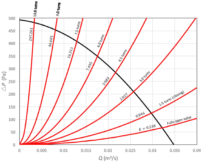
 : system curves. Each curve in this family is the result of a different degree of valve opening. The slope of the curves increases as the valve is closed. Each curve has its correspondent loss coefficient for reference;
 increases slightly with Reynolds number. It is hence not surprising that the error increases with flow rate.
 , in equation (1).
 (11)
(11) is the channel's width and
  and
and  are the upstream and downstream depths respectively.