Continuous Measurement of Biological Noise in Escherichia Coli Using Time-lapse Microscopy

Summary

This work presents a microscopy method that allows live imaging of a single cell of Escherichia coli for analysis and quantification of the stochastic behavior of synthetic gene circuits.

Abstract

The protocol developed here offers a tool to enable computer tracking of Escherichia coli division and fluorescent levels over several hours. The process starts by screening for colonies that survive on minimal media, assuming that only Escherichia coli harboring the correct plasmid will be able to thrive in the specific conditions. Since the process of building large genetic circuits, requiring the assembly of many DNA parts, is challenging, circuit components are often distributed between multiple plasmids at different copy numbers requiring the use of several antibiotics. Mutations in the plasmid can destroy transcription of the antibiotic resistance genes and interject with resources management in the cell leading to necrosis. The selected colony is set on a glass-bottom Petri dish and a few focus planes are selected for microscopy tracking in both bright field and fluorescent domains. The protocol maintains the image focus for more than 12 hours under initial conditions that cannot be regulated, creating a few difficulties. For example, dead cells start to accumulate in the lenses' field of focus after a few hours of imaging, which causes toxins to buildup and the signal to blur and decay. Depletion of nutrients introduces new metabolic processes and hinder the desired response of the circuit. The experiment's temperature lowers the effectivity of inducers and antibiotics, which can further damage the reliability of the signal. The minimal media gel shrinks and dries, and as a result the optical focus changes over time. We developed this method to overcome these challenges in Escherichia coli, similar to previous works developing analogous methods for other micro-organisms. In addition, this method offers an algorithm to quantify the total stochastic noise in unaltered and altered cells, finding that the results are consistent with flow analyzer predictions as shown by a similar coefficient of variation (CV).

Introduction

Synthetic biology is a multidisciplinary field that has emerged in the past decade and aims to translate engineering design principles into rational biological design^1,2,3, in an effort to achieve multi-signal integration and processing in living cells for understanding the basic science^4,5, diagnostic, therapeutic and biotechnological applications^6,7,8,9,10. Our ability to quantify the input-output response of synthetic gene circuits has been revolutionized by recent advances in single-cell technology, including the flow analyzer and live cell imaging using automated time-lapse microscopy¹¹. A flow analyzer is often used to measure the response of these circuits at the steady state^1,12, and inverted microscopy is used to measure the dynamic response of synthetic gene circuits at the level of a single cell³. For example, one of the early works in synthetic biology involved the construction of genetic oscillator networks in living cells using negative feedback loops with a delay³. Later on, the genetic oscillator circuits were applied to understand metabolic control in the dynamic environment of living cells⁴. Automated time-lapse microscopy is one method to characterize such circuits. We hypothesize that the host cells, Escherichia coli, synchronize when forming micro colonies, allowing measurement of signal and calculation of noise without tracking exact mother-daughter relations.

Noise is a fundamental, inherent aspect of biological systems often arising from multiple sources. Consider for example, biochemical reactions involving signals that originate from the transport of discrete random carriers such as diffusion of proteins¹³. These signals propagate with random fluctuations¹⁴. Other noise sources are resource availability, cell division and variations in environmental conditions such as temperature, humidity and pressure. Biological signals that propagate in synthetic gene circuits often have a very low signal to noise ratio (SNR), which disturbs the performance of such circuits. Therefore, genetic circuit design remains one of the most challenging aspects of genetic engineering¹⁵. For example, in contrast to most approaches which calculate only the mean gene expression (measured over the entire cell population), the variance of the measured signal is considered in order to engineer predictable behavior through synthetic gene networks¹². As such, the levels of variability or noise in the protein expression play a dominant role in design and performance of analog and digital gene circuits^1,16,17.

Many approaches has been developed to quantify cell-to-cell variability, including in Escherichia coli^3,7,18. These methods are often used to study gene activation and metabolic pathways, however with less focus on the study of stochastic noise dynamics, like measuring and disentangling specific noise sources, especially for genetic circuits in living cells where this is a fundamental challange^19,20,21. Several factors, both inherited to the circuit itself (intrinsic) and derived from the host cells (extrinsic), can disturb the continuous performance of genetic circuits. In this paper, we developed a protocol that aims to quantify the total noise in Escherichia coli cells, including the intrinsic and extrinsic noise sources^6,22. By quantifying the total noise and then evaluating the SNR²³, the design of gene circuits can be improved. This method can be modified to measure independent noise sources separately, by monitoring several fluorescent proteins^6,20. For the protocol described here, we keep the environmental conditions well controlled and continuously measure the activity of cells without the influence of external factors. We measure the signal from fluorescent proteins in single cells over time and simultaneously image them under an agarose substrate. The resulting images are analyzed using the laboratory's custom MATLAB.

Ideally, continuous measurement of the real time activity of fluorescent proteins inside a cell will produce accurate data through the growth and division of the cells. However, it is challenging to acquire such data. This is due to degradation of fluorescent proteins, known as photo-bleaching⁷, when they are exposed to radiation in the excitation process. Furthermore, Escherichia coli cells are also sensitive for the excitation, which might lead to phototoxicity⁷. Both issues limit the amount of photo frames that can be acquired and the time between acquisitions. The substrate and medium types (e.g., lysogeny broth) that is used to grow the cells during imaging also have a critical role. We strongly recommend using minimal medium, which minimizes non-fluorescent background and extends cell division time.

Moreover, the sample needs to be prepared considering the following requirements (1) Low cell division rate allows for less frequent exposures for closely imaging the division cycle and reducing the probability of phototoxicity and photobleaching. We set the acquisition time to about half of the predicted mitosis time (2) Low cell density at the beginning of the experiment allows for better uniformity and trackability of division. Cell density is affected by the dilution ratio of the Escherichia coli cells, which is a significant parameter for the success of this protocol and needs to be determined for every lab. In order to establish the ratio, each new Escherichia coli strain or media used should be fitted with growth rate graphs (Supplementary Figure 1). An appropriate ratio has been achieved if cells can grow without additional shaking after a short incubation from an initial density of about OD_600nm = 0.1. Cells at this phase will divide according to the environment temperature only (3) Restriction of cell movement: cell movement strongly depends on substrate (agarose pad) firmness. The substrate firmness depends on the amount of total agarose and the gel solidification time. Gels cannot be left to solidify overnight at room temperature, as the Escherichia coli will undergo mitosis. Other factors that affect substrate stability include the amount of water in the sample and humidity. Additional issues are discussed in detail in the Representative Results. This protocol provides many details and gradually moves from one step to another. The protocol offers long stability for imaging experiments and provides a basic image processing tool. 

Protocol

1. Media and culture preparation

1. Prepare stock solution of 1,000x Carbenicillin (50 mg/mL) or relevant antibiotic.
   1. .Weigh 0.5 g of carbenicillin. Add 10 mL of sterile H₂O. Dissolve completely.
   2. Sterilize carbenicillin stock through a 0.22 µm syringe filter. Aliquot the antibiotic solution and store at -20 °C.
2. To prepare lysogeny broth (LB) plates, mix 5 g of tryptone, 5 g of NaCl, 2.5 g of yeast extract and 7.5 g of Bacto agar with 0.5 L of sterile H₂O. Autoclave the solution at 121 °C for 20 min.
   1. Partially submerge the molten gel-mix in a 50 °C water bath.Add 1,000 µL of carbenicillin (50 mg/mL).
   2. Prepare Petri dishes in a sterile environment. Leave the plates to set before storing them in the fridge.
3. For M9 minimal media, prepare separate stock solutions of the following: 5x M9 salts (56.4 g/L), 2 M glucose and 2% biotin-free casamino acids. Autoclave the solutions at 121 °C for 20 min.
4. To prepare 5 Petri plates, mix 1125 mg of low melting agar and 400 mg of agar with 89.2 mL of minimal media (1x M9). Add 10 mL of 2% casamino acids (2% [vol/vol]) in a 250 mL Erlenmeyer flask.
   NOTE: Make sure to pour the media on the inner lips of the flask.
5. Microwave the solution in short bursts of 3 to 4 seconds. Repeat until the solution is clear.
   NOTE: Make sure not to reach boiling point.
6. Place the 250 mL Erlenmeyer flask in a hot water bath (60 °C) to further mix by diffusion, and leave it to cool until its temperature falls to about 45-50°C.
7. Light the flame at the plate-pouring bench.
8. Add quickly all the solutions in the following order:
   800 µL of 50% glycerol (0.4% [vol/vol])
   100 µL of thiamine (B1)
   1100 µL of Glucose (2M)
   100 µL of Carbenicillin (50 mg/mL).
9. Swirl the Erlenmeyer flask to ensure even distribution of all ingredients throughout the agar.
10. Open one plate at a time next to the flame and begin pouring.
    1. Leave the plates on the bench for a few minutes until initial solidification.
    2. Turn the plates upside down to prevent water condensation from dripping onto the gel.
    3. Leave the plates to solidify at room temperature for about 2 h.
    4. Once the plates have solidified and dried, they can be stored at 4 °C for about 3 months.

2. Bacterial strains and plasmids construction

NOTE:The genetic circuit contains one part; a Green Fluorescent Protein (GFP) driven by a P_tetO promoter resulting in constitutive expression. All the plasmids in this work were constructed using basic molecular cloning techniques and were transformed into Escherichia coli 10β, using a standard heat shock protocol²⁴. The final construct was transformed into Escherichia coli MG1655 wild type strain for testing.

1. Transform the desired plasmid into Escherichia coli MG1655 cells with the standard heat shock protocol²⁴.
2. Grow the transformed cells on an LB agar plate overnight at 37°C.
   NOTE: It is possible to keep the Petri dishes from step 2.2 up to 3 days for microscopy use.
3. Inoculate a single colony into 5 mL of LB broth supplemented with the relevant antibiotics in a glass tube.
4. Grow cells at 37 °C with 250 rpm shaking speed in incubator for 2 h until liquid is cloudy.
5. Prepare 1 mL of dilution solution as follows:
   892 µL of minimal media (1x M9)
   8 µL of 50% glycerol (0.4% [vol/vol])
   100 µL of 2% Casamino acids (0.2% [wt/vol])
   1 µL of thiamine (B1)
   11 µL of Glucose (2 M)
   ​1 µL of relevant antibiotics
   1. Mix and spin down.
6. Dilute the cell culture (1:30) from step 2.4 into a 2 mL tube by adding 30 µL of Escherichia coli growth to 1000 µL of dilution solution (step 2.5).
7. Incubate the tube for 1 h with shaking (250 rpm) at 37 °C.
8. Grow 40 µL - 60 µL on M9 plates prepared in step 1.10. Incubate the plate at 37 °C overnight.
   NOTE: The Optical Density (OD_600nm) for plating should be around 0.1.
9. Place up to three 35 mm glass bottom plates on the bench.
   NOTE: Make sure the plate's glass has the correct thickness for the microscope lenses used.
10. Prepare the culture for seeding on gel plates, repeat steps 2.3 to 2.6 for colonies from plate prepared at step 2.9 microscope measurements.
11. Prepare the following solution to make three microscope plates.
    1. Preheat the water bath to 60 °C.
    2. Mix 112.5 mg of low melting agar and 40 mg of agar with 8.92 mL of minimal media (1x M9) and add 1 mL of 2% casamino acids (0.2% [vol/vol]) in a 25 mL Erlenmeyer flask.
       NOTE: Make sure to pour the media on the inner lips of the flask.
12. Microwave the solution in short bursts of 2 to 3 seconds. Repeat until the solution is clear.
    NOTE:Make sure not to reach boiling point.
13. Place the 25 mL Erlenmeyer flask in a hot water bath (60 °C) to further mixing by diffusion, and leave it to cool on the bench until its temperature falls to about 45-50 °C.

3. Preparation of agarose pads

1. Clean bench with 70% ethanol. Stretch tape on the cleaned bench. Make sure the tape is smooth and leveled.
2. Prepare two coverslips: one on the tape and a second one nearby. Prepare a coverlid.
3. Remove flask (prepared at step 2.14) from water bath, wipe the outside of the flask clean and leave it to cool until its temperature falls to about 45-50 °C.
4. To make the gel solution, mix quickly all the solutions in the following order:
   80 µL of 50% glycerol (0.4% [vol/vol])
   1 mL of 2% casamino acids (0.2% [wt/vol])
   10 µL of thiamine (B1)
   110 µL of glucose (2 M)
   10 µL of relevant antibiotics.
5. Pour 1.5 mL of the gel on the coverslip and cover it with the second piece making a "sandwich".
6. Return the Erlenmeyer to the hot water bath. Cover the sandwich with the lid and set timer for 20 minutes.
7. At the same time, incubate the tube from step 2.11 for 1 h at 37 °C with shaking (250 rpm)
8. After 20 minutes flip the sandwich (step 3.5), cover it and leave to rest for 1 h.
   NOTE: For better results leave the "sandwich" to rest at 4 °C for the duration of step 3.8.
9. Seed Escherichia coli culture from step 3.7 by pipetting the sample onto the 35 mm dish.
   NOTE: Pipetting 6 µL of cells as separate small drops gives the best results.
10. Allow the drops to dry, for at least 15 minutes and up to 30 minutes.
11. Expose the solidified gel of the sandwich from step 3.8 by sliding the coverslip away.
12. Cut sandwich into small individual pads with biopsy punch or tip.
13. Lean it gently on the sample (step 3.9). Leave the dish for 20 minutes on the bench.

4. Preparing the sample for microscopy imaging

1. Remove the flask from water bath from step 3.6. Wipe the outside of the flask clean and let cool to room temperature (25 °C).
   NOTE: Remove the flask at step 4.1 about 3 minutes before the timer ends.
2. Pour 3 mL of the gel constantly to the plate perimeter in a circular motion. Leave to solidify for a few minutes.
3. Seal plates with tape and pierce several holes with 25 G needle. Flip all the dishes to prevent water condensation dripping onto the gel.
4. Incubate all the dishes at 4 °C for 30 min to allow full solidification while preventing cell mitosis.
   NOTE: Leave samples at 4 °C for successive measurements, no more than one day.
5. Start the microscope per manufacturer instructions.
6. Find the initial focus using lowest amplification lens and engage automatic focus system (AFS).
7. Use oil if needed, drown the lens with oil and spread it carefully by moving the plate with a platform controller (not manually) and AFS can be engaged again.
8. Use relative cross-section in Z direction, following default suggestion for Z step cross-sections.
   NOTE: We took bright field images every 5 minutes and fluorescent images every 20 minutes. Sometimes the focus needs to be adjusted during the first 30 minutes. Preheating the microscope incubator box and oil, while refrigerating the sample tends to help reduce the initial loss of focus.

5. Data analysis

NOTE: In order to process microscopy data, we designed a computer-based software in MATLAB. This software facilitates identification of cell boundaries from bright field tiff images and segments and sorts cells by area. The output of this image analysis can be used as a mask on fluorescent tiff images to derive cell intensity levels and cancel artifacts in the fluorescent domain such as cell halo due to microscope resolution limits. The software developed was inspired from similar works^{7,25,26,27,28,29,30} and provides an elegant solution tailored for the lab.

1. First, define the following parameters in main_code.m.
   1. Define the folder of the acquisition images.
   2. Define the image time period - bright field channel time step in minutes.
   3. Define the GFP frequency - rate of acquisition of GFP images.
   4. Define the microscope resolution (i.e., how many pixels equals 1 µm).
   5. Define histogram bin range - cell area range.
      NOTE: The process of classifying the data according to cell area is similar to the principles of gating in flow cytometry data analysis. Gates are placed around populations of cells with common characteristics, usually forward scattered and side scattered, to isolate and quantify these populations of interest. Microscopy allows to gate, investigate and quantify several cell groups.
   6. Define convolution kernel (3,3) - this parameter detects cell boundaries by global thresholding (count_cells.m).
      NOTE: This setup is needed only when changing the lab or microscope. Software requires the input bright field channel to be labeled with index c1, fluorescence channel labeled as c2.
2. Run main_code.m, which will run all other scripts automatically (count_cells.m, cell_growth_rate.m).
   1. Program automatically segments bright field images (see Supplementary Figure 2-4).
   2. Combine the segmentation image with fluorescent image (GFP) to extract intensity level per cell.
   3. Calculate the graph of amount of cells by time and fit according to exponential growth.
   4. Calculate the mean and standard deviation (STD) for each cell area range.
   5. Calculate the signal to noise ratio (SNR) for each cell area range.
   6. Plot and fit the distribution of amount of cells by intensity.
   7. Calculate the coefficient of Variance (CV) and compare to flow analyzer data.
      NOTE: Software will give as output the final segmentation images for adjusting conv_kernel in a new folder "yourfolder/Segmented". Software will give as output the graphs in a new folder "yourfolder/Graphs.
3. In order to compare between experiments, use compare_experiments.m.
   1. Define directories for the saved graphs and the address for the \CompareResult directory.
   2. Run the file.

Representative Results

The software analyzes bright field domain images that are off-white and black. The Escherichia coli will look like black oblong shapes on an off-white background and dynamic range of luminance should show a spike at its center (Figure 1). In fluorescent images cells may have a small halo but individual cells with oblong shapes can still be resolved. A mitosis event should be first detected after 30 minutes. Microscope focus should remain stable over time and although cells might move slowly during those 30 minutes, they are unlikely to leave the field of view. Such an experiment will be considered good and can be viewed at Figure 2. Cells might be hard to detect in the bright field domain at low magnification. We recommend establishing the average focus distance with a high copy number (HCN) plasmid, as it is easy to notice at low magnification. Set the average distance while measuring a low copy number (LCN) plasmid at the high magnification in advance. This focus distance depends mainly in the plates, the microscopy system and oil, and not the thickness of gel or Escherichia coli strain.

When adapting this protocol to other labs, the following issues may arise (1) Escherichia coli plates (samples) prepared at an incorrect dilution ratio can show unchanging numbers of cells (Figure 3 and Figure 4) (2) Samples prepared without sealing the plate can show excessive shrinkage. This can be observed as cells drift (Figure 3) or cause a loss of focus (Figure 5) (3) Some samples may exhibit slow shifting 'fixed' cells (in black) on a background of swimming cells (in white). This is likely due to a wet sample and it usually stabilizes as the excess water is absorbed by the gel (Supplementary Video 1) (4) Samples that exhibit no cells after a few minutes of warming up might have been prepared incorrectly, likely due to: (I) Gel was poured while still too hot, (II) protective cap was forgotten, (III) minimal media lacks an ingredient, (IV) incorrect cell density, and (V) gel was sealed too tightly. It is important to punch holes to allow gas exchange at the expense of gel shrinkage (Figure 5) and (VI) cells can also indent the gel in search for nutrients, stacking one on top of the other, compromising the cell monolayer effectively preventing detection of cells and measuring of reliable fluorescent signal (Supplementary Figure 5).

We have measured three circuits in this work. First, a constitutive promotor that regulates GFP shown in Figure 6. Second, a constitutive promotor that regulates super-fold GFP³¹ (sfGFP) shown in Figure 7. An ssrA degradation tag (AAV) was added to sfGFP to reduce itshalf-life to minutes⁵. The third circuit is based on a positive feedback circuit¹, and is induced by acyl-homoserine-lactone (AHL). The P_luxR promoter regulates sfGFP and LuxR, a transcription factor binding with AHL to activate P_luxR as shown in Figure 8. Figure 9 presents the dynamics of cell growth (cell numbers versus time), Figure 10 shows the dynamics of the measured signal (mean fluorescence versus time), and Figure 11 shows dynamics of evaluated total noise (standard deviation (STD) versus time).

The SNR (or CV) is widely used in designing analog electronic circuits to express the precision and reliability of the circuit³². CV relates to the distribution of signal between single cells and allows comparison across methods and different equipment such as microscopes and flow analyzers. Calculating SNR from microscope images allows us to compare circuits across time, segmented cells are measured at the same time as providing a measure for the specific resolution of the noise compared to the signal, or a noise interval for a specific time and inducer concentration. This may indicate if detector cells will be able to resolve the exact signal response to the inducer concentration. In this work, the CV was calculated by considering all segmented artifacts which are cells, regardless of the cell progression in the division cycle. SNR was calculated for specific cell area range over time, and then it was averaged for three repeated experiments. Neither the acquired signal nor the STD are reliable alone, as they are specific to the experiment and equipment used. The signal is measured with arbitrary units which depends on equipment gain preset, photo-detector and exposure time. The data presented in Figure 10 suggest that the cells stage in the division cycle does not affect the noise level, as different ranges of area (points in the division cycle) show the same trend. This observation might support the claim that tracking exact mother - daughter relations can be avoided for measuring noise and this could improve the SNR for the presented method. No substantial change in SNR was observed between GFP to sfGFP as shown in Figure 12. We calculate the SNR (SNR= mean/ STD) and present it in Figure 12 and Figure 13.

We then calculated the variance and CV based on the following equations³¹

1.1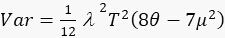 

1.2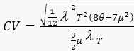 

Where λ is protein folding time, T is cell division time, θ and µ are the number of plasmids before and after division, the plasmid copy number³¹. Using the above equations (1.1, and 1.2) we can fit the data from the flow analyzer signal for gamma distribution.

Then we compared between the CV, which is measured and calculated by flow analyzer (Figure 14), and by the protocol (Figure 15).

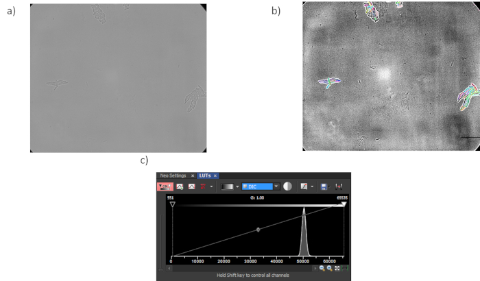
Figure 1: Bright field exposure image (a) Stabilized acquisition in bright field (b) Segmentation image, only colored cells enter the calculations (c) Pixel brightness map of the acquisition, spike is the background noise. Thresholding by it segments only Escherichia coli. Please click here to view a larger version of this figure.

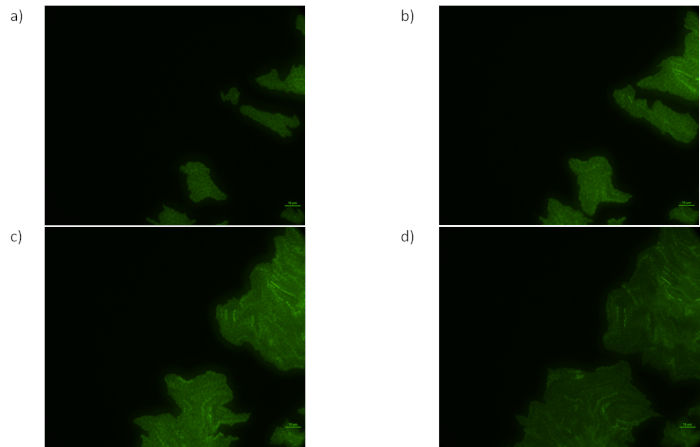
Figure 2: This experiment shows good healthy cells dividing and reacting after 120 minutes. Images were acquired successively at 20 minute intervals. Colonies are in focus, gel is stable between samplings. Colonies divide and produce strong signals. Please click here to view a larger version of this figure.

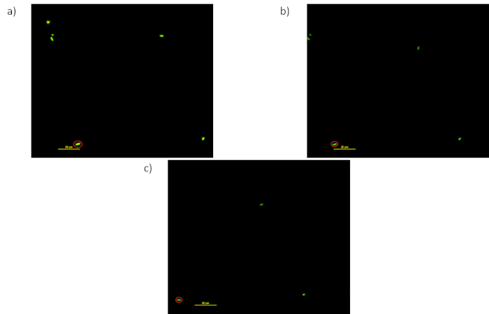
Figure 3: Effects of incorrect dilution ratio and gel shrinkage on fluorescent image. Images were acquired at 20 minute intervals (a) Individual Escherichia coli circled in red (b) The same cell drifts to the right of the field of view (c) The cell drifts further. The cells also do not divide or change positions, probably due to a low dilution ratio and gel shrinkage. Please click here to view a larger version of this figure.

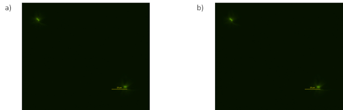
Figure 4: In this experiment no activity was detected and almost no cells were present. Possible reasons are the gel being too hot, the drying of the sample being too aggressive or having no protective cap (a) Fluorescent images taken at 40 minutes (b) Fluorescent images taken at 60 minutes. Please click here to view a larger version of this figure.

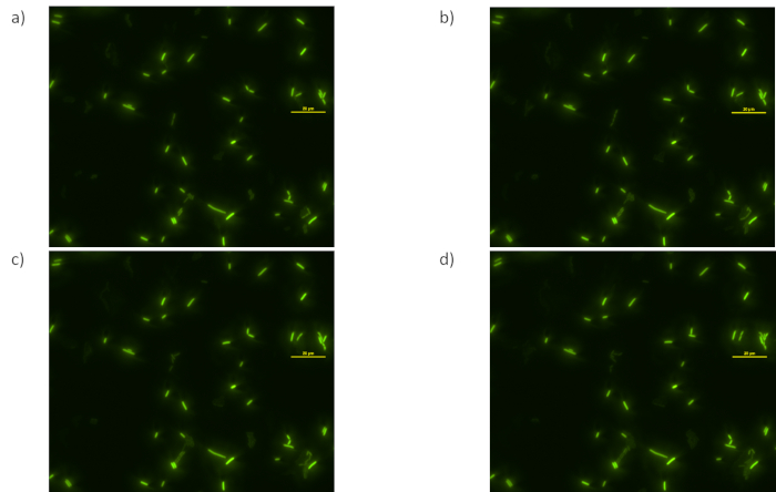
Figure 5: Focus loss and photobleaching.Successive images of (a) through (d) were acquired at 15 minute time intervals using auto focus system. See Supplementary Video 2. Please click here to view a larger version of this figure.

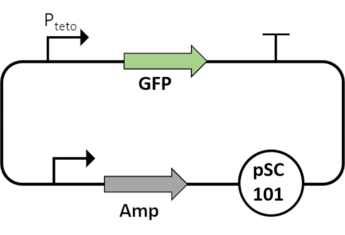
Figure 6: Plasmid map of P_teto that regulates GFP. Without the TetR repressor, the P_tetO promoter acts as a constitutive promoter. The circuit is cloned on low copy number plasmids. This plasmid acts as a basis for SNR measurement for any modified circuit. Please click here to view a larger version of this figure.

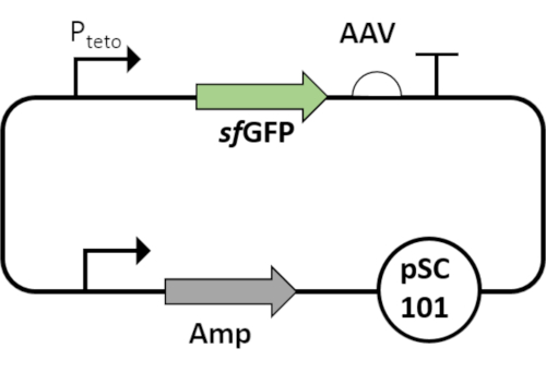
Figure 7: Plasmid map of P_teto that regulates sfGFP. The sfGFP is fused to an AAV degradation tag. The circuit is cloned on low copy number plasmids. The sfGFP-AAV is a more robust variant of GFP, while the AAV tag rendering it susceptible to degradation by housekeeping proteases of the Escherichia coli. Please click here to view a larger version of this figure.

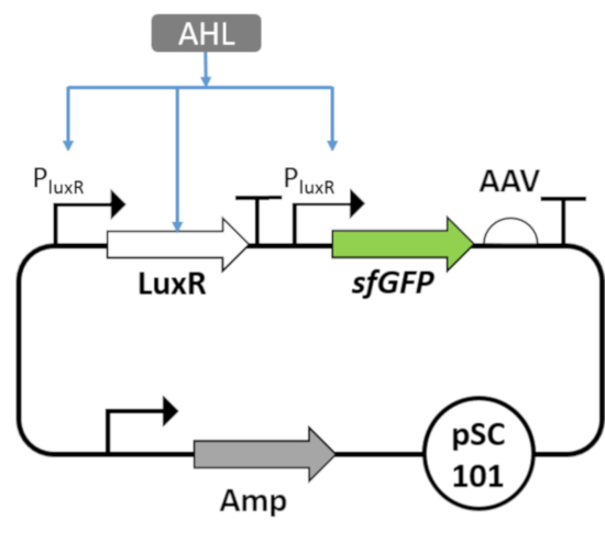
Figure 8: Plasmid map of positive feedback circuit. The circuit is induced by an AHL inducer, which binds LuxR transcription factor. The P_luxR promoter, which is regulated by AHL-LuxR complex, actives the production of LuxR and sfGFP-AAV. The circuit is cloned on low copy number plasmids. Please click here to view a larger version of this figure.

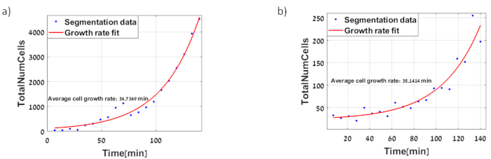
Figure 9: Dynamics of Escherichia coli MG1655 strain growth in minimal media includes (a) P_tetO-GFP, exponential growth of about 35 minutes. The images of this experiment are shown in Figure 2 (b) P_tetO-sfGFP, exponential growth of about 35 minutes. Please click here to view a larger version of this figure.

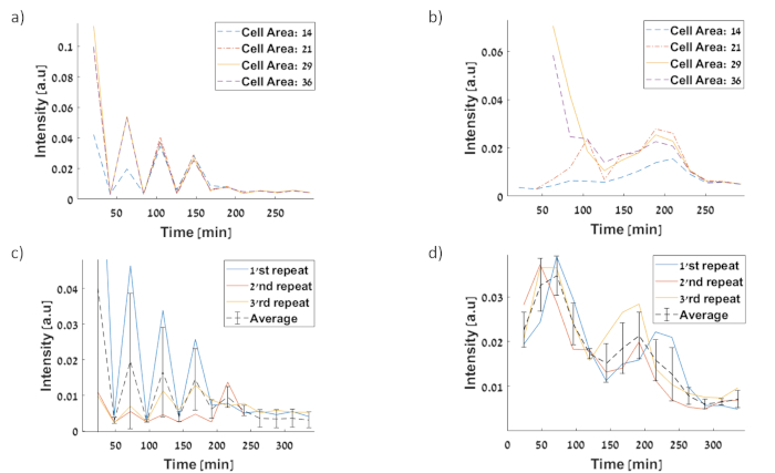
Figure 10: Fluorescent intensity level, normalized per pixel and acquired at 20 minute intervals. 
Cells are binned according to area, in order to minimize artifacts. Cells are divided by their area in a micrometer square (a) P_teto-GFP circuitfirst repetition for intensity at 210 minutes is 0.004 a.u (b) P_tetO-sfGFP circuit first repetition for intensity at 210 minutes is 0.022 a.u (c) Measured signal of P_teto-GFP circuit (d) Measured signal of P_tetO-sfGFP circuit. All experimental data represents the average of three experiments. The software can sort cell area to different groups (a) and (b) show graphs for four cell area ranges representing the division cycle. First area of 14 micrometers represents cells after division as most likely that cells after division will be the smallest. The second area of 21 µm represents cells before division. Third and fourth areas represents cells at division as the total area is multiplied by two (29 and 36 µm) in order to consider cells that took longer to divide. The areas were chosen by manually assessing the data looking on microscopy images. Please click here to view a larger version of this figure.

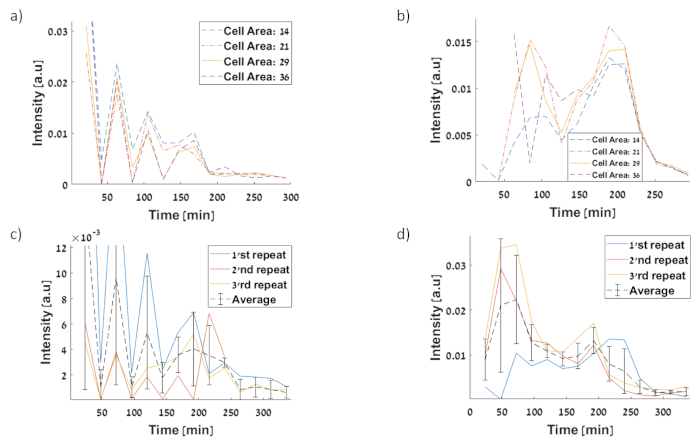
Figure 11:Standard deviation (STD) of single cell fluorescence intensities for: (a) P_tetO-GFP circuit first repetition for STD at 210 minutes is 0.001865 a.u (b) P_tetO-sfGFP circuit first repetition for STD at 210 minutes is 0.01477 a.u (c) STD of P_teto-GFP circuit (d) STD of P_tetO-sfGFP circuit. Please click here to view a larger version of this figure.

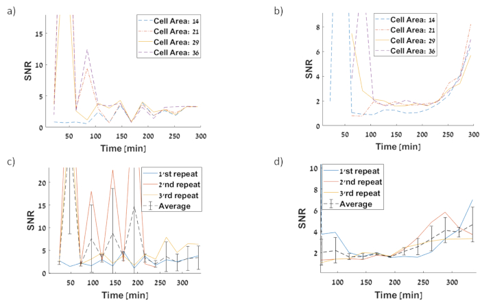
Figure 12:SNR of single cell fluorescence intensities. We calculate the SNR=Mean/STD (a) P_tetO-GFP circuit first repetition for SNR at 210 minutes is 1.309 a.u (b) P_tetO-sfGFP circuit first repetition for SNR at 210 minutes is 1.29 a.u (c) Three repetitions of GFP measurement (d) Three repetitions of sfGFP measurement. Please click here to view a larger version of this figure.

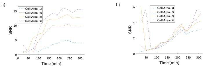
Figure 13:SNR of single cell fluorescence intensities (a)P_luxR-sfGFP circuit SNR for saturation response to AHL (b) P_luxR-sfGFP circuit SNR for half time response to AHL. The SNR of positive feedback AHL regulated circuit is higher than SNR for constitutive sfGFP circuit. Please click here to view a larger version of this figure.

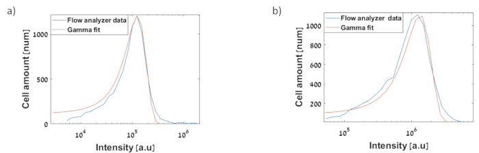
Figure 14: Histograms of the gene circuits based on the flow analyzer: experimental data (blue) and stochastic model data (red). The x axis represents arbitrary fluorescence units from flow cytometry, and the y axis represents the frequency of cells producing the corresponding fluorescence level. The data was measured using a flow analyzer after three hours. GFP fluorescence was quantified by excitation at a wavelength of 484 nm and emission at a wavelength of 510 nm. PE-TexasRed filter voltages were used on a high throughput sampler to measure GFP expression levels. The flow analyzer voltages were adjusted using software so that the maximum and minimum expression levels could be measured with the same voltage settings. Thus, consistent voltages were used across each entire experiment. The same voltages were used for subsequent repetitions of the same experiment. Fitting was made by use of gamma distribution³¹. This method assumes that the signal depends mostly on random distribution of plasmids (a) Measurement of P_teto-GFP clone on low copy number plasmid. Experimental CV=0.46, Model CV=0.32 (b) Measurement of P_teto-sfGFP-AAV cloned on low copy number plasmid. Experimental CV=0.86, Model CV=0.44. Please click here to view a larger version of this figure.

Figure 15: Histograms of the gene circuits based on microscope: experimental data (dotted lines) and stochastic model data (solid lines). The x axis represents arbitrary fluorescence units from inverted microscope and the y axis represents the frequency of cells producing the corresponding fluorescence level. Fitting was made using the MATLAB gamma distribution^31,32 (a) Measurement of P_tetO-GFP clone on low copy number plasmid (b) Measurement of P_tetO-sfGFP-AAV cloned on low copy number. Comparison shows that our protocol obtains similar CV values as in flow analyzer experiment. Please click here to view a larger version of this figure.

Supplementary Figure 1: Four dilution ratios, between 1:500 and 1:20, for the MG1655 strain. The graph shows that if initial density is high, LB nutrients are abundant resulting in cells dividing faster. For a 1:500 dilution, cell density remained constant. For a 1:100 dilution, cell density increased slowly. For a 1:50 dilution, cell density increased at moderate division rate without significant delay in 250 RPM incubation. For a 1:20 dilution, the cell density reached saturation fast. We chose a dilution ratio of 1:30, allowing short incubation for reaching exponential growth and substantial division range for achieving high saturation at moderate division rate. Please click here to download this figure

Supplementary Figure 2: Processing bright field images. (a) Raw data intensity images from the bright field channel from the microscope system. (b) Contrast enhancement manipulation of the image to improve separation of cell objects from the background. (c) Cell boundary recognition based on convolution filter³³ and binarization based global threshold³⁴. (d) Morphological³⁵ operations of closing and filling to identify cell colony boundaries. Please click here to download this figure

Supplementary Figure 3: Cell colony background\foreground segmentation. To minimize the impact of the noise we try to identify cell colony boundaries and extract them from the gel noise. (a) Image binarization operation on contrast enhancement based on adaptive thresholding to detect cell objects³⁶. (b) Matrix multiplation of matrixes presented at S2d and S3a successfully filtering out most noises and differentiating gel noise from cells. Some boundries are not fully resolved. (c) Identification of cell boundaries using a watershed algorithm³⁷ based on distance transform³⁸. (d) Matrix multiplation of matrixes presented at S3b and S3c successfully resolving single cells. Please click here to download this figure

Supplementary Figure 4: Single cell segmentation. (a) Segmented product of bright field image. Further cleaning is preformed based on cell area gating and shape, discarding round bubbles. (b) Fluorescence signal images acquired from microscope. (c) Matrix multiplation of matrixes presented at S4a and S4b successfully extracting the signal of single cells. Please click here to download this figure

Supplementary Figure 5: Loss of monolayer. (a) Bright field image of a cell layer at 840 minutes (14 hours) of P_teto that regulates GFP circuit shown in figure 2 in the article as a good experiment. At the right side of microscopy image loss of monolayer can be detected. (b) Software segmentation image. Due to loss of monolayer cells are fragmented and will be cleaned base on area gating. (c) Fluorescence image showing that on the right side of image no cells can be resolved and a low signal of cells on the left side of the image due to loss of monolayer. (d) Segmentation image combined with fluorescence image. Please click here to download this figure

Supplementary Video 1. Please click here to download this video

Supplementary Video 2. Please click here to download this video

Supplementary Video 3. Please click here to download this video

cell_growth_rate_fit.m.  Please click here to download this file

compare_experiments.m.  Please click here to download this file

Count_Cells.m.  Please click here to download this file

main_code.m.  Please click here to download this file

Discussion

In this work, we developed a protocol that enables computer tracing of Escherichia coli live cells, following division and fluorescent levels over a period of hours. This protocol allows us to quantify the stochastic dynamics of genetic circuits in Escherichia coli by measuring the CV and SNR in real time. In this protocol, we compared the stochastic behaviors of two different circuits as shown in Figure 10. It has been shown that plasmids with low copy numbers are more prone to stochastic effects and less affected by cell division. The first circuit constitutively expressed GFP (Figure 10a), and the second circuit constitutively expressed sfGFP fused to a ssrA degradation tag (Figure 10b). In order to quantify the stochastic behavior of the fluorescent proteins, we also recorded the bright field images. The results show that the expression of GFP, specifically at its maturation³⁹, is the dominant noise source. The periodic saw tooth behavior pattern observed in Figure 10a can be explained by the random process of cell division and the long-time scale of GFP maturation (~50 minutes). By contrast, the sfGFP signal of the second circuit was stabilized during the measurement, because the very short maturation time of the sfGFP (~6 minutes). We developed a simple formula that describes the level of GFP in both circuits when we consider only the process of cell division and GFP maturation time. At a given time, t, we assume that there are x copy numbers of proteins, and µ copy numbers of plasmids. The protein copy number can be described by:

1.3 

1.4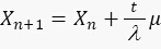 

When considering only division events;  after protein maturation and so for the specific plasmids we get:

For GFP (): 1.5 

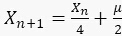
For sfGFP ():1.6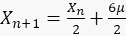 

Then, the developed series of sfGFP:

1.7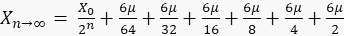 

In the case that , we obtain . This result can be explained as follows. When x is small, sfGFP levels increase by a small amount. When x is large, sfGFP is degraded to a steady state. Similarly, for the circuit of GFP, each cell contains about 10 units of GFP, but since maturation time for GFP is longer than the mitosis, degrading saw tooth patterns of fluorescence intensities are observed. In the model, we assumed that replication of the plasmid is fast enough that plasmid distribution remains constant before and after division. The ssrA degradation tag often reduces the protein half-life time from hours to less than an hour⁵ and leads to a fast steady state. We showed that the method also provides a distribution similar to that measured with a high population flow analyzer and that the CV of this distribution is equal to or smaller than the flow analyzer CV.

While several methods^3,7,18 were developed for live cell imaging, the method presented here is tailored specifically to Escherichia coli. This bacterium requires a special media and a slightly different approach. The protocol has the following important features: (1) Establishing a dilution ratio specific to the bacteria and strain at the beginning of exponential growth rather than at the middle stage (Exponential growth without shaking) (2) Escherichia coli best divide at 37 °C, but at 37 °C the minimal media gel loses water rapidly which leads to shrinkage and instability. The protocol here overcomes this challenge (3) We first apply the bacteria sample and then seal it with liquid gel. Since the sample is trapped between the glass bottom and gel we require a gel that (I) allows gas exchange to avoid cutting air pockets, (II) remains liquid at low temperatures as Escherichia coli are sensitive to heat and (III) makes sure the sample will not be mixed inside the liquid gel. The gel remains liquid at 37 °C, however, we recommend use of a protective cap on top of the sample to avoid excessive heat and sample mixing inside the gel (4) This approach requires simple, generic equipment (5) Samples can be measured directly without preheating, so there is no loss of division events (6) The protocol, which includes the wet-lab steps and the customized automated software, can be used to study the stochastic behavior of genetic circuits such as quantifying the SNR and CV of circuit signals. We compared the microscopy method to flow analyzer results in order to validate the use of small populations of cells and establish a baseline for comparison according to CV (7) The software allows us to detect cells on the monolayer without human intervention and analyze total noise. Software tools such as ImageJ¹⁸ or Schnitzcells require manual identification of cells and are challenging for adjustments.

When continuously imaging living cell colonies, design the experiment while considering several complex physical parameters, such as cellular stress and toxicity, rate of resources depletion, necrosis and degradation time of inducers and chemicals. The protocol allows reliable measurement of up to five hours. Our experiments suggest that Escherichia coli synchronize when dividing in micro, monolayer colonies (Supplementary Video 3). We assume that the gel is uniform in terms of resources and toughness, the cells have similar behavior, and the field of illumination is slightly bigger from the field of view. Thus, each cell should produce the same signal and statistical data, which can be collected as we have shown by comparing CV obtained in this way to measurement with a flow analyzer. In order to measure noise at constant initial conditions for longer periods of time, we will consider using microfluidic chips in the future. Further benefits of such a device are maintaining fixed positions of cells and stable focus¹⁰. Still, design, fabrication of microfluidic chips and priming for experiments require training, specific equipment (custom made at times) and time. For this reason, it is beneficial to use time lapse microscopy as shown in this protocol to acquire a general understanding of the circuit.

The proposed protocol and the developed software allow reproducible measurements, from which it is simple to derive graphs. It also allows testing and comparison of total noise and can be modified for measuring intrinsic and extrinsic noise. The method is based on generic or easy to order materials, openly shared, easy to use software and does not require specific training. We have shown that the population measured by microscopy is big enough to obtain meaningful data by comparing the method CV to that obtained with a flow analyzer. Therefore, we can successfully establish a SNR baseline using this protocol and compare it to more complex gene circuits.

Materials

Name	Company	Catalog Number	Comments
35mm glass dish	mattek	P35G-0.170-14-C	thickness corresponding with microscope lense.
Agarose	Lonza	5004	LB preperation
AHL	Sigma-Aldrich	K3007	inducer
Bacto tryptone	BD - Becton, Dickinson and Company	211705	LB preperation
Carb	Invitrogen	10177-012	antibiotic
Carb	Formedium	CAR0025	antibiotic
Casamino acids	BD - Becton, Dickinson and Company	223050	minimal media solution
eclipse Ti	nikon		inverted microscope
Glucose	Sigma-Aldrich	G5767	minimal media solution
Glyserol	Bio-Lab	000712050100	minimal media substrate
Immersol 518F	zeiss	4449600000000	immersion oil
M9 salt solution	Sigma-Aldrich	M6030	minimal media solution
NaCl	Bio-Lab	214010	LB preperation
Noble agar	Sigma-Aldrich	A5431	minimal media substrate
parafilm tape	Bemis	PM-996	refered to as tape in text
Seaplaque GTG Agarose	Lonza	50111	minimal media substrate
thaymine B1	Sigma-Aldrich	T0376	minimal media solution
Yeast Extract	BD - Becton, Dickinson and Company	212750	LB preperation