Rodent Estrous Cycle Monitoring Utilizing Vaginal Lavage: No Such Thing As a Normal Cycle

Summary

This study details the crucial factors to consider in experimental designs involving female rats. In a larger sense, these data serve to decrease stigma and assist in the development of more inclusive diagnostic and intervention tools.

Abstract

The current methodology establishes a reproducible, standardized, and cost-effective approach to monitoring the estrous cycle of female Sprague Dawley (SD) adolescent rats. This study demonstrates the complexity of hormonal cycles and the broad spectrum of understanding required to construct a reliable and valid monitoring technique. Through an in-depth examination of principal experimental design and procedural elements, this description of the cycle and its fundamental principles provides a framework for further understanding and deconstructs misconceptions for future replication.

Along with an outline of the sample collection process employing vaginal lavage, the procedure describes the mechanism of data categorization into the four-stage model of proestrus, estrus, metestrus, and diestrus. These stages are characterized by a new proposed approach, utilizing the 4 categorizing determinants of vaginal fluid condition, cell type(s) present, cell arrangement, and cell quantity at the time of collection. Variations of each stage, favorable and unfavorable samples, the distinction between cyclicity and acyclicity, and graphic depictions of the collected categorizing components are presented alongside effective interpretive and organizational practices of the data. Overall, these tools allow for the publication of quantifiable data ranges for the first time, leading to the standardization of categorization factors upon replication.

Introduction

Novel contributions
The rodent estrous cycle has been identified as an essential indicator of wellness. However, unconscious biases of investigators and inaccurate interpretations regarding the female body hinder the scientific community. The very etymology of the word "estrous" implies a sense of inferiority and negativity. Euripides used the term to describe a "frenzy" or madness, Homer to describe panic, and Plato to describe an irrational drive. This study highlights how these primeval perspectives influence the current scientific community and addresses these concerns through a novel mosaic paradigm—an updated combination of previously studied methods, expanded in scope for a more comprehensive approach.

The study and use of this technique are necessary, first, as there is no standardized and comprehensive monitoring technique, and data interpretation practices can be unclear. Second, although estrous cycle characteristics are dependent on individual rats being studied, they are often universalized. Third, while hormonal cycles are routine and beneficial processes, they are surrounded by hazardous stigma explored in the 'Translation to Humans' section. This study aims to address these three issues in three ways—(A) by describing an in-depth estrous cycle monitoring technique and clarifying how the results can be interpreted, (B) by outlining methods that maintain the integrity and individuality of each cycle, and (C) by calling attention to misconceptions that perpetuate unsubstantiated practices.

This study is also unique in its focus on adolescent rats, a period marked by crucial developmental changes that shed light on various behavioral, anatomical, and physiological manifestations in adulthood¹. Building a standardized experimental design to monitor hormonal cycles in an under-researched population while deconstructing common biases will allow for the development of reliable and valid hormonal correlations^2,3,4 and the determination of condition-dependent cycle disruptions^5,6,7,8,9,10. Ultimately, these novelties serve to expand diagnostic criteria, treatments, and interventions of various wellness concerns.

Fundamental definitions and uses
The estrous cycle is a collection of dynamic physiological processes that occur in response to the three oscillating female sex steroid hormones: estradiol, leuteinizing hormone (LH), and progesterone (Figure 1A,B). Interactions between the endocrine and central nervous system regulate the cycle, which most often persists for 4-5 days and recurs from the onset of sexual maturation until reproductive senescence and/or cessation. It is divided into separate categories based on hormone levels—most commonly into the 4 stages of diestrus (DIE), proestrus (PRO), estrus (EST), and metestrus (MET), which progress in a circular fashion. The number of divisions can range from 3 stages¹¹ to 13 stages¹², depending on the nature of the study¹³. The lower number of divisions often excludes MET as a stage and classifies it as a short-duration transitionary period. The higher number typically includes subsections that allow for a closer inspection of phenomena such as tumor development or spontaneous pseudopregnancy, the physiological state of pregnancy without embryonic implantation^12,14,15.

In this study, the stages were identified through components of the vaginal canal, named the 3 categorizing determinants-cell type(s) present, cell arrangement, and cell quantity (Figure 2A-D). While the condition of the vaginal fluid was not monitored in this study, it is recommended to include it as a fourth categorizing component. Further information on examining the vaginal fluid can be found in the reference list¹⁶. The categorizing components can be examined by extracting cells via vaginal lavage, the primary technique recommended in modern-day estrous cycle monitoring. While the in-depth physiological processes within each stage are outside the scope of this study, more information can be found in the literature¹⁷.

The use and continued development of this estrous cycle monitoring technique is rooted in the connections between sex steroid hormones and the function of bodily systems such as the cardiovascular system¹⁸, endocrine system⁸, and central nervous system^19,20,21. At the same time, estrous cycle monitoring may not always be necessary when female rodents are involved^22,23,24,25. Rather, it is important first to consider if sex differences have been reported in the specific area of study, which can be further explored in published reviews^22,23. Though estrous cycle monitoring is vital in a broad spectrum of research investigations, it should not be seen as an obstacle to including female rodents in experiments. While this technique may appear complex and time-consuming, the procedure itself can take less than 15 min to complete, depending on the investigator, and is cost-effective. Overall, the inclusion of female rodents in scientific studies is advantageous to the understanding of bodily systems, various conditions and pathologies, and general wellness, as these developments have been mainly based on the male body template.

Universal parameters and natural variabilities in the rodent
Establishing ranges for aspects seen as "typical" is necessary to define standard cycle patterns, set parameters for comparative and analytic purposes, and detecting abnormalities and outliers. At the same time, it is also important to recognize that each rat's cycle is unique, and deviations based on animal strain, physiological processes, and environmental conditions are expected. In fact, one of the most "normal" aspects of the estrous cycle is variability. This is seen in the total cycle length, with a range of 3-38 days^26,27; the age of sexual maturation that can range from 32-34 days to multiple weeks^28,29,30; what is considered acyclical¹¹, and the categorizing determinant patterns^11,13. Overall, there is no universal template for the estrous cycle, and translating that to both the scientific community and the general public is an important part of the experimental process.

Experimental timepoints and developmental age
Recognizing this principle of variability assists in building a reliable and valid experimental design. For example, the start of estrous cycling monitoring relies on the rats' anatomical and physiological development, which varies based on environmental and physiological factors. Monitoring cannot begin until the development of the vaginal opening (VO), which is the external vaginal orifice surrounded by the vulva that leads to the interior portion of the vaginal canal (Figure 3A-D). While the VO often fully develops between the ages of 32 and 34 days, it remains individualized to each subject, and much about the process remains unknown. This opening has been used to identify the onset of sexual maturation, which has been linked to the increase of estradiol³¹, the maturation of the hypothalamic-pituitary-ovarian axis³², and the first ovulation in rats^{17, 33,34,35}. However, recent publications have found that it is only an indirect marker of reproductive development, as it can become uncoupled from hormonal and developmental occurrences in unfavorable environments³¹ and may represent changes in estradiol levels rather than sexual maturation³³. Therefore, it is recommended to not rely solely on the VO to determine developmental age and as a qualifier for estrous cycle monitoring³⁶ but to also utilize the appearance of the first EST stage and cornification of the epithelial cells³⁰ to mark the onset of sexual maturation.

Body weight is notably correlated with developmental age during the adolescent period in rodents^30,37 and can therefore also assist in determining developmental age in this period. Proposed mechanisms related to this phenomenon include the stimulation of hormones necessary for reproductive development, such as growth hormone, and the inhibition of the hypothalamic-pituitary adrenal (HPA) axis by the appetite regulator, leptin³⁰. However, it is not recommended to utilize this measure as the sole indicator of developmental age due to the large variance seen between rats across species and vendor providers³⁸. The variability seen in the development of the VO and body weight exemplify the importance of the concept in the overall experimental process.

Translation to humans: cultural and scientific contexts
The translational relationship of animal-to-human reproductive studies is bidirectional. The results from animal-based studies influence how the human processes are assessed, approached, and analyzed³⁹. The perception of the human reproductive system and its related processes influence how animals are studied. In fact, one of the loudest indications for further research in this area stems from biased sociocultural beliefs related to hormonal cycles that influence the scientific process. Many of these conventions are derived from a general cultural aversion to discussing menstruation, which has led to a data gap in well-substantiated knowledge^40,41. This has a spectrum of consequences that span from minor to lethal—from shelving height and smartphone size to police body armor fitting and missed cancer diagnoses⁴².

The description of menstruation as unsanitary, destructive, and toxic—seen in revered texts, media, dictionaries, and medical teachings—is conserved by scientific publications. This occurs through inaccurate and biased descriptions of hormonal cycles, the isolation of the reproductive system from its neuroendocrine counterparts and environmental influences, and the reductionist perspective of the completion of a cycle as a 'failure to conceive'^43,44. This leads to the creation of unsound experimental practices, such as the omission of external variables that influence hormonal cycles, determining start and endpoints based solely on anatomical developments, and measuring cycle advancement in a linear rather than circular fashion. Despite the direct correlation between sociocultural factors and biological consequences, it is not often considered in scientific literature. Through the inspection of more holistic publications^43,44,45, researchers can deconstruct these stigmas and create more reliable and valid experimental designs.

Protocol

All handling and procedure methods outlined in this protocol align with National Institutes of Health (NIH) animal care and use guidelines and have been approved by the Institutional Animal Care and Use Committee (IACUC) of Pepperdine University and The UCLA Chancellor's Animal Research Committee (ARC).

1. Animal care and use

1. Acquire female rats, in numbers according to power analysis, and male rats to promote the Whitten effect or more consistent cycling⁴⁶. Determine the strain based on the objective of the study in known databases⁴⁷.
   NOTE: The current data reflect that of female adolescent SD International Genetic Standardization Program (IGS) in the presence of male SD rats located at both Pepperdine University and UCLA laboratories as part of a collaborative study. These rats arrived in separate groups at 28 days of age, and the estrous cycle progression was monitored for either 10 or 20 days to demonstrate differences on acute and chronic levels, beginning at 34 days of age (following a 7-day acclimation period).
2. Before handling, allow for a quarantine and/or an acclimation period for physiological stabilization following transportation and adjustment to the new environment.
   NOTE: A 3-day minimum period has been cited, with a 7-day period recommended^{48,49,50,51,52}. Overall, this is dependent on the transportation conditions, animal strain, and study objectives.
3. Ensure that stress is reduced with the use of an acclimation period, as stress can disrupt proper reproductive system functioning⁵³. However, do not overcompensate by attempting to eliminate it, as a moderate amount of stress is beneficial to the animals' well being⁵¹.
4. Host rats in a temperature- (68-79 °F, i.e., 20-26 °C) and humidity-controlled (30-70%) environment by contacting the vivarium or laboratory managers and ensuring these features. Distribute water and chow ad libitum with nutrient components listed on the company website and cage cleaning once a week.
   NOTE: In this study, the rats were housed in groups of 2 separated by sex in 19" x 10" x 8" clear reusable plastic cages and had access to corncob bedding that was changed once a week. The temperature was maintained at 70 °F and humidity at 35-79%, with an average of 62%.
5. Check for the development of ringtail or ischemic necrosis of the tail and toes for evidence of low relative humidity levels and extreme temperatures, which may cause the alternation of biological responses.
   NOTE: Temperature and humidity are important for the reproductive system, sexual maturation, and estrous cyclicity^{54,55,56,57,58}.
6. Ensure proper and balanced illumination throughout the housing space by depositing equal amounts of light sources throughout the laboratory space that act on a time-controlled light:dark system.
   NOTE: Here, a 12:12-h light:dark cycle, with lights on from 06:00-18:00 h, was controlled by 2,550-lumen Linear LED bulbs.
7. Follow lux requirements provided⁵² based on variations of animals' pigmentation, age, strain, sex, and hormonal status.
   ​NOTE: When researchers categorize the cell samples collected, consistent lighting will allow for proper visual detection and reliable staging⁵⁹. The duration and intensity of light are directly related to the reproductive system, sexual maturation, and estrous cycling^{54,55,56,57,60,61}.

2. Equipment and experiment preparation

1. Review the categorizing determinants (seen in Figure 2A): how to identify each stage of the estrous cycle and how to operate the microscope and camera equipment.
2. Ensure that each subject to be monitored has reached sexual maturation and shows appropriate indicators of development—VO, body weight, and age. Weigh the rats and examine them for VO between at the same time each day for accurate comparisons and transfer them with an approved handling method. Consult the university-affiliated veterinarian if an animal loses more than 20% of its previous body weight.
   NOTE: The VO remains caudal to the urethral opening and cranial to the anus, located between the two, as depicted in Figure 3.
3. As these factors are strain-dependent, check with the supplier for specifications and consider environmental factors specific to the laboratory⁶².
   NOTE: In general, this will occur between 32-34 days of age and an average body weight ranging from 75-150 grams⁶³ for SD rats and is indicated by a circular-shaped opening previously covered by a membranous sheath.
4. Select a sample collection period appropriate for the group of rats being monitored to prevent collecting transitional samples. First, sample a few animals at 2 or 3 different timepoints throughout the day to determine the time where most cycle stages are present (e.g., sampling at 12:00 hours, 13:00 hours, and 14:00 hours for different animals). Complete the vaginal lavage at the same time each day for consistent and reliable staging.
   NOTE: It has been reported that the hours between 12:00 and 14:00 h are best for capturing all stages. In this study, estrous cycle monitoring occurred between 12:00 and 14:00 h, handled with the compression-style hold (see step 3.4). The importance of estrous cycle monitoring timing relative to other experimental interventions (e.g., behavioral conditioning, medication) is a developing area of research and can be further explored¹¹. Determining the duration of the estrous cycle monitoring is study-dependent and can be further explored in published studies^11,33.
5. Remove the protective cover from the microscope and attach the camera to the computer by removing the protective camera lens cover and placing the lens over the eyepiece of the microscope.
6. Then, open the preselected software on the computer. To use the software selected in this study, select the camera attached to the USB located on the left-hand side of the screen, under the tab labeled Camera List. Ensure that the USB camera is properly connected to the computer, which will read No Device under the tab labeled Camera List, if not.
7. Once the USB camera has been selected under the tab, turn on the microscope light switch located on the base.
8. Create a folder on the computer designated for the cell sample photos. Create a file folder for each separate day that data are collected, preprepared before images are taken.
9. With the equipment prepared, retrieve the subject's cage from its holding place and bring it to the sample collection station.

3. Collection of vaginal cells

1. Retrieve a disposable syringe and fill each of the syringes with 0.2 mL of sterile 0.9% NaCl. If air bubbles are present, gently flick the barrel syringe until all the air bubbles have reached the open tip of the syringe and expel the air. If there are still air bubbles present, expel the solution back into the NaCl receptacle and refill until there are none.
   NOTE: Excessive flicking may result in the formation of more air bubbles.
2. Return each syringe to the plastic wrapping to maintain a sterile field, with the tip of the syringe inside the sealed portion of the wrapping.
3. Open the cage and gently lift the subject by either the base of the tail or the trunk of the body, closing the lid of the cage to prevent others from exiting. Select a holding method from those listed below based on personal preference and animal response.
4. Use the compression-style hold for adolescent rats by placing the subject against the upper chest region, with the subject's nose pointing down at the ground. Before beginning the swab, ensure that the subject is compressed enough to prevent movement but is comfortable and safe in the hold. Expose the vaginal canal of the subject by gently flexing the tail before inserting the syringe.
5. Use the Hind Leg Lift for adult rats by placing the animal's forepaws on either the top or side of the cage, while the tail and hindlimbs are restrained with a gentle hold between the first and second fingers, leaving the thumb free to operate the syringe⁶⁴.
6. Allow for the animals to acclimate to the handling and monitoring. Handle the animals gently yet securely to reduce excess stress and to protect the researcher from aggression such as biting.
   NOTE: The first few days of monitoring may not produce the desired results as the animals acclimate to their conditions. Handling the animals to collect body weights during the acclimation period can assist this transition³³.
7. While holding the syringe steady with the forefinger and middle finger, insert the tip of the syringe (no more than 2 mm) at an angle parallel to the vaginal canal. Slowly expel the NaCl into the canal by pushing the plunger inwards. Do not insert the syringe further into the canal, as doing so may disrupt the estrous cycle.
8. Extract the NaCl from the vaginal canal by pulling the plunger of the syringe away from the epithelial lining (upwards). If there is difficulty keeping the subject in the hold during this process, place them back into the cage for a short rest period before attempting NaCl extraction.
9. Once the cell sample has been collected, place the subject back in the cage and repeat this procedure for each animal before all samples are evaluated under the microscope.
   ​NOTE: Alternatively, each sample can be collected and evaluated before moving on to the next animal. An animal may require a second lavage if the sample cannot be categorized. The same syringe from the initial collection can be reused if it does not contact the saline directly in the container and only for the same animal.

4. Sample evaluation

1. Begin the categorization by examining the vaginal fluid sample extracted. Record the viscosity as either viscous or nonviscous and the coloration as either opaque or transparent on the description document or other recording system.
   NOTE: This section of the protocol can be performed at the time of sample collection or later.
2. Expel 2-3 drops of the fluid onto a microscope slide and place a microscope cover glass on top of the slide. Place the cover glass on the microscope slide from the top of the slide to the bottom or from one side of the slide to the other to prevent the formation of air bubbles. If possible, leave approximately half of the collected sample in the syringe if further examination is required and to prevent an excess amount of fluid from being placed on the slide.
3. Locate the cells collected by moving the microscope slide across the stage. If there are too few cells or a high amount of debris, expel the remaining fluid onto a new slide and reexamine. If the amount of sample left in the syringe is insufficient, or if the second drop is presenting similar issues, collect another sample from the subject before attempting to identify the estrous cycle stage.
4. Once the cells have been located and before touching the computer or the computer keyboard, remove the one glove to prevent soiling the keyboard.
5. Acquire images of the cell samples by clicking on the function labeled Snap on the left-hand side of the software panel.
6. Then, save the file by clicking on Save as under the File icon on the top left corner of the page. Save the photo under a prelabeled folder on the computer.
   NOTE: Example label template: #subjectnumber_date collected_estrous stage_objective lens used.
7. Take more than one photo at each objective lens if there are not many cells within each frame.
   NOTE: Example labels for multiple images: #1_01/09/2021_EST_4x1 and #1_01/09/2021_EST_4x2.
8. Repeat the procedure for each collected sample under multiple objective lenses. Include at least one smaller objectification, such as 4x, and at least one larger objectification, such as 20x.
9. Upload the images to a shared drive/folder or an external hard drive so all researchers involved have access to the files and there are backup copies available.

5. Stage categorization

1. Set up the computer screen to simultaneously view the photos taken and the recording sheet (Figure 4A-C).
   NOTE: This will allow for the documentation to occur while viewing the sample collected. This portion of the protocol can be completed at the time of sample collection or later.
2. Determine which cell types are present in the sample. Select from the four options listed in steps 5.2.1-5.2.4 using the criteria and record the findings.
   1. Anucleated keratinized epithelial (AKE)/cornified epithelial cells
      1. Look for jagged or angular-edged cells, as seen in Figure 2B and Figure 5C, which despite the lack of nuclei, may show light round areas (nuclear ghosts) within the cell that represent where a nucleus was once present. Use higher magnification, such as 20x and above, to differentiate between such nucleated and anucleated cells.
      2. Use higher magnification to distinguish the keratinized or cornified portion of the cell—a thin layer of cells lacking nuclei and filled with keratin—if desired.
         NOTE: In addition to their jagged appearance, these can also be distinguished by how they can fold or disassemble, creating jagged and elongated structures known as keratin bars.
   2. Large nucleated epithelial (LNE) cells
      1. Look for these typically round- to polygonal-shaped cells encased by irregular, jagged, or angular borders.
      2. Observe how their nuclei may take on various forms, ranging from intact to degenerate or pykontic, relating to the irreversible condensation of chromatin in the nucleus of a cell undergoing death or deterioration, as seen in Figure 2B and Figure 5D1,2. Take note of how these nuclei occupy less space than the cytoplasm within the cell, with a lower nuclear to cytoplasmic (N:C) ratio than the small epithelial cells. Look out for cytoplasmic granules that can be seen at higher magnifications¹³.
   3. Leukocytes (LEUs)/neutrophils/polymorphonuclear cells
      1. Look for these compact, spherical cells with multilobulated nuclei (hence, known as polymorphonuclear cells), which vanish as the cell matures (Figure 2B and Figure 5A). Higher magnification (e.g., 40x) can be used to observe the multilobulated nuclei.
         NOTE: Upon collection and preparation, these cells may condense, fold, or rupture.
   4. Small nucleated epithelial (SNE) cells
      1. Look out for these round- to oval-shaped cells that are larger than the neutrophils described above.
      2. Observe the round nuclei of these nonkeratinized epithelial cells (Figure 2B), which take up a larger amount of space than the cytoplasm inside the cell, creating a higher N:C ratio relative to large epithelial cells.
         NOTE: Upon collection and preparation, these cells may fold or overlap to create a shape that resembles a string or bar, as demonstrated in Figure 5B1.
3. Examine how the cells present in the sample are organized for each objectification. Use the lower objectification, such as 4x, to view a representative view of the overall cell arrangement. Record whether the cells are clumped together (C), evenly dispersed (ED), or randomly dispersed (RD) (see Figure 4C), and note the specific organization of each cell type (e.g., small nucleated epithelial cells are clumped, and neutrophils are evenly distributed).
4. Next, visually estimate and record the total cell quantity (a smidge, moderate, numerous) and the individual cell quantities (percentage of each cell type present).
   NOTE: A smidge represents the smallest number of cells present that can be utilized to determine the sample categorization, numerous represents the presence of a countless number of cells that either account for most if not all of the space on the slide or are stacked on top of one another, and a moderate number of cells represents a comparatively average number of cells (examples seen in Figure 5A-D and Figure 6A-D).
5. Note whether there are any deviations from either the listed criteria or aspects that are typical for the specific subject in the 'abnormalities' category and consult with a veterinarian if needed.
6. Determine which estrous cycle stage is being presented in the sample utilizing the categorizing components and the descriptions below.
   1. DIE
      1. Look for LEUs as the dominant or only cell type present, arranged in a clumped manner at the beginning of DIE but more dispersed in late stages.
         NOTE: While transitioning into DIE, the quantity of cells may decrease as the epithelial cells begin to break down, as seen in Figure 6D1. At the same time, the number of LEUs begins to increase, and they tend to be arranged in a clumped manner initially and disperse over time.
      2. Note that the total quantity of cells may be comparatively low, most often in the later stages of the DIE period, on the second or third day.
      3. Observe the high amount of mucus that may be present in this stage, which presents as concentrated strands of LEUs (Figure 5A1). Look out for small clumps or cellular strands of SNE cells accompanying the LEUs during late phases in the transition to PRO (Figure 5A1,2).
      4. Observe the viscous and opaque appearance of the vaginal fluid when transitioning into, fully transitioned into, and transitioning out of DIE.
         NOTE: The average duration of this stage is 48 h during a 4-day cycle and possibly 72 h during a 5-day cycle.
   2. PRO
      1. Look for SNE cells as the dominant cells and for LEUs, LNE, and/or AKE cells that can be seen in low numbers. Use high objectification to observe the granular appearance of the SNE cells that are typically arranged in clusters, sheets, or strands during this stage (Figure 5B1,2).
      2. Observe the viscous and opaque appearance of the vaginal fluid when moving from DIE into PRO, and how it becomes nonviscous and transparent once fully transitioned into the PRO stage (average duration of 14 h in rats).
   3. EST
      1. Look for dominance of AKE cells, a diminishment of the SNE cells in EST, and an increase in the number and size of cells as EST continues^11,13.
      2. Make a note of the distinguishing feature of the often clustered arrangement of AKE cells, in the form of keratin bars or containing ghost nuclei, which can become more randomly dispersed in the transition from PRO (Figure 6B) and to MET (Figure 6C).
      3. Observe the characteristic nonviscous and transparent vaginal fluid, which can be expected as the rats are transitioning into, fully transitioned into, and transitioned out of EST.
         NOTE: The progression of EST includes much diversification (Figure 5C and Figure 6B, C). The stage typically occurs for an average of 24 h in a 4-day cycle or possibly 48 h in a 5-day cycle.
   4. MET
      1. Look for higher numbers of SNE and LNE cells as the rat is transitioning into MET, either dominant in terms of cell proportion within the canal or close to equal proportion to the LEUs^11,13. Further, make a note of the greater amount of debris in MET and the transitions than in other stages due to the epithelial cell decay following EST and moving into DIE.
      2. Observe the lack of consistent arrangement as all cell types are seen and in various amounts (Figure 5D1-3). However, look for the LEUs that are packed or clumped in proximity to the epithelial cells in the beginning stages that may return to the clumped arrangement when transitioning into DIE.
      3. Observe the nonviscous and transparent appearance of the vaginal fluid in this stage and the change to a more viscous and opaque appearance while moving into DIE.
         NOTE: The average duration of this stage is 6-8 h.
7. Label samples in transitions with the stage the subject is moving towards, with the transition in parenthesis to track when these are collected. Further information on how to distinguish between these 4 stages and their transitions can be found in the Representative Results.
   NOTE: As the samples collected are static and the cycle is dynamic, the slides may depict transitions between stages (seen in Figure 6A-D).
8. Complete this process for each animal until the monitoring phase is complete.
9. On either day 11 (45 days of age) or 21 (55 days of age), euthanize the rats with 5% isoflurane and 2% oxygen before a guillotine decapitation. These timepoints may vary depending on the nature of the study.

Representative Results

The current data reflect that of female adolescent SD International Genetic Standardization Program (IGS) in the presence of male SD rats. These animals were located at both Pepperdine University and UCLA laboratories as part of a collaborative study. Figure 5 presents multiple variations of the 4 cycle stages. Figure 5A1 was identified as a diestrus sample with several cell types present. This example demonstrates that samples with a larger number of epithelial cells qualify as diestrus when they meet the other categorizing component qualifications, such as a dominance of LEUs. This sample also demonstrated the mucus strand arrangement composed LEUs often seen in this stage, which resembles the strands consisting of SNE cells seen in the PRO stage. To distinguish a mucus strand in the DIE stage from the strands that appear in the PRO stage made up of SNE cells, it is important to identify the dominance of LEUs. Figure 5A2,3 display a cell arrangement progression often observed—an initial clumping of the LEUs that collect and move to a random (RD) or even disbursement (ED) in samples collected in later periods of the DIE stage. Specifically, Figure 5A2 was a DIE sample with numerous cells present. This reflects how the LEUs may also be accompanied by a high number of epithelial cells (Figure 5A1,2), distinguished from metestrus by a dominance of LEUs and the absence of keratin bars. In contrast, Figure 5A3 demonstrates that a low total cell count (a smidge) was commonly seen during the later phase of the DIE stage, such as during the second or third day. During the PRO stage, the SNE cells were frequently arranged into strands with numerous cells stacked on top of one another (Figure 5B1) or a smidge of cells arranged into smaller clumps (Figure 5B2). Figure 5B3 exemplifies a PRO sample with the characteristic sheet-like clumping of SNE cells that overlap and form bars that could be confused with the keratin bars composed of AKE cells present in the EST stage. To distinguish the two, it is important to identify the dominance of SNE cells in PRO and of AKE cells in EST.

Figure 5C1,2 demonstrate the typical clumping and random disbursement of AKE cells seen in EST, with the former including numerous cells and the latter a moderate number. Ghost nuclei, keratin bar formations, and bacteria often collected during this stage are seen in these examples. SNE cells were at times represented during the EST stage (Figure 5C1) as remnants of the previous PRO stage. The late EST stage, when SNE cells begin to emerge as the subject moves towards MET, is often mistaken for the PRO stage. To distinguish the two, it is important to take the nuclear size into account. In general, the nucleated cells of PRO have a higher N:C ratio. The sample shown in Figure 5C3 presented a strand-like arrangement of numerous AKE cells that was not seen as a characteristic of the EST stage. This demonstrates that each animal is unique, that deviations from the criteria may occur, and that the categorizing determinants are to be examined in combination.

To distinguish between EST and PRO when SNE cells are present, it was seen that a lower N:C ratio occurred in these cells during the EST stage. To distinguish the keratin bars present in EST from those formed by the overlapping or rolling of SNE cells in the PRO stage (Figure 5B3) and those formed by decaying epithelial cells in the transition from MET (Figure 6D1), it is important to identify the dominant cell type, arrangement, and quantity to distinguish the stage being represented. Lastly, Figure 5D1,2 exemplifies the combination of all cell types present in the random disbursement representing the MET stage. In addition to the numerous cells present in these examples, it was common to collect a higher amount of debris during this stage (Figure 5D2) due to the decay of epithelial cells following EST and the transition into DIE with a dominance of LEUs that function to clear the vaginal canal of epithelial cells. Figure 5D2 also displays how MET can be distinguished from DIE by its higher concentration of epithelial cells and the presence of keratin bars. Overall, these representations depict the broad spectrum that exists within each stage and are nonexhaustive.

Representations of the 4 transition phases are shown in Figure 6. While this study categorized samples in transition as one of the 4 estrous cycle stages, it remains important to identify the transition phases properly. In the transition from DIE into PRO (Figure 6A), there was often an overall decrease in the number of LEUs and an increase in the number of SNE cells. LNE and AKE cells were at times present in this transition, though not in high amounts (Figure 6A1). Figure 6A2-4 depict the higher number of clumped and randomly dispersed SNE cells that were often collected during this transition, with a low number of randomly and evenly dispersed LEUs. Overall, when distinguishing from other transition stages, it was important to note the dominance of SNE cells and the beginning of clumps and strand formations seen in PRO. All examples in Figure 6A represent a numerous cell count except Figure 6A4, with a smidge. In Figure 6B, the image shows an example of numerous clumped SNE and AKE cells that are seen in the transition from PRO to EST.

During this transition, SNE cells are seen to be in higher numbers with less clumped and more random disbursements of AKE cells than during EST. Figure 6C shows the emergence of AKE, SNE, and LNE and the decrease in AKE cells in the transition from EST to MET with a high number of cells. The debris present represents the decaying AKE cells from the previous estrus stage often seen in metestrus. This is also seen in the final transition stage, from MET to DIE, where the epithelial cells began to decay and produce debris (Figure 6D1,2), with numerous cells present in the former and a moderate number in the latter. These figures display the phenomenon of LEUs increasing in number to become the dominant cell type in the transition to diestrus. For the group monitored for 20 days (n = 3), there were 12 days when transition samples were collected, with an average of 4. For the group monitored for 10 days (n = 3), there were 9 days when transition samples were collected, with an average of 3.

Figure 7 represents unfavorable cell sample collections, a majority of which warranted repeat lavages. Figure 7A1 shows a mass of squamous cells collected due to an improper syringe insertion and extraction, causing squamous cells to be suctioned off the vaginal canal wall. These cells can be distinguished from clumped epithelial cells or LEUs due to the high density and compactness of the mass and its distinctive borders. Figure 7B represents a collection of debris, where either no cells were extracted, the plane of focus is incorrect, or the slide was not fully scanned for cells. Debris can be distinguished from cells through familiarity with the cell types and the often distinctive small size and clumping. This debris often stems from animal bedding, hair, or cell decay. Figure 7C depicts a slide that contains a cell count that is below a smidge. While low cell counts were commonly seen during late MET and early DIE, this represents slides that have too few cells to accurately categorize into a stage.

Figure 7D shows two examples of the NaCl extraction solution combined with vaginal fluid from the canal on the microscope slide. In the first image, Figure 7D1, the fluid was present and out of focus, obstructing the ability to accurately categorize. In Figure 7D2, the fluid was spread across the slide in cohesive circles alongside the LEUs. While this example does not require a repeat lavage due to the high cell presence, it is important to consider the quantity of fluid placed on the slide and the placement of the microscope cover slide to prevent smears. Overall, these images emphasize the importance of capturing quality representative images for proper categorization. This includes considering the manner of cell extraction, the plane of focus, and the content of the image by scanning each slide before capturing an image.

After categorizing each animal in the experimental group(s), it is common to graph the stage progressions on either a bar or line graph. This allows researchers to examine the overall cycle pattern and identify when the animal presents an irregular progression of the estrous stages, known as acyclicity. The samples can then be analyzed by the cycle length and stage progression pattern in this analysis tool. Shown in Figure 8A,B, this concept includes assigning bars of varying heights, in the case of this study, to the individual stages and translating the recorded data (Figure 4B) across the x-axis. In these examples, MET and DIE are represented by the lowest, PRO by the middle, and EST by the tallest bar heights. Due to the short duration of the MET stage, it is combined with the DIE stage into one bar. Though there are different methods of measuring cycle completions, it is common to count one complete cycle as the movement from one EST to another¹¹. However, this does not reflect a cycle completion but a 2-day EST stage duration when there are consecutive EST stages.

Figure 8A reflects data from a rat that progresses through a consistent and repetitive progression through MET/DIE, PRO, and EST. Additionally, this rat fell within the range of 4- to 5-day cycles at an average length of 4.375. Each stage does not exceed the standardized ranges of length, with an average of 1.0625 days spent in EST, a typical evaluation for acyclicity. If the data extracted follow this pattern of EST to EST with regularity, this confirms not only that the subject's hormone levels remained within acceptable ranges, but also that the procedure was conducted without significantly interrupting the cyclical nature of the process. Lastly, this rat completed 16 cycles, determined by counting the number of EST to EST bars.

Figure 8B represents common types of acyclicity, including extended (seen as EXT) and unrecorded stages. This figure also highlights the importance of examining both the cycle pattern and the length and number of days spent in each stage. Specifically, in this example, while the average cycle length and number of days in EST fall within outlined parameters, the cycle pattern of stage progression revealed abnormalities. Therefore, it is important to examine the estrous cycle comprehensively. Both extended DIE (labeled as Ext Diest) and EST (labeled as Ext Est) stages were recorded throughout the cycles shown in the figure, and there were multiple cycles where the PRO stage was unrecorded. This example also demonstrates the importance of examining the number of consecutive stages seen, which fall outside typical ranges, rather than solely examining the average length of the cycle and days in EST, which fall within typical ranges.

The causes and correlations of these examples can include factors such as physiological abnormalities (tumors, pseudopregnancy, prolonged stress), harmful environmental conditions (prolonged illumination, exposure to toxic chemicals, solitary housing), improper timing of sample collection, researcher error (poor sample collection, image capture, improper staging), age-related phenomena (common irregularity seen in adolescence and reproductive senescence), or deviations unique to the specific animal. To separate researcher error or improper timing of sample collection and physical abnormalities or age-related phenomena, it is helpful to examine the 4 categorizing components in greater detail. This can assist in determining the possible causes of irregularities or, in a broader sense, could be utilized in studies that are studying the estrous cycle characteristics more closely.

Figure 9 illustrates this closer inspection by including total and individual cell quantities on the y-axis, cell type(s) represented by different bar fill colors, and cell arrangement(s) represented by different bar fill patterns, graphed across the total monitoring period. This analysis method allowed for the examination of the total number of cycles completed, the length of each cycle, stage progression, and the categorizing components in greater detail for each individual rat. Figure 9A represents a rat that had a lower than average number of cycles, with a total of 3 full cycles in the 10 days monitored-two 3-day cycles and one 5-day cycle (average of 3.67). The irregularity seen in the stage progression with 50% of the days included one or more unrecorded stages and 30% of samples collected being in transition-—day 2 as a MET-DIE, day 5 as an EST-MET, and day 8 as a PRO-DIE transition. This could have been due to the improper timing of sample collection, researcher error, an age-related phenomenon, or unique deviations. Further monitoring could have provided clarity as to which applied.

The typical dominant arrangements, cell types, and individual and total cell quantities were seen within each of the stages recorded. Within the EST stages, a smidge (25% of samples), moderate (25% of samples), and numerous (50% of samples) clumped AKE cells were seen, with a lower presence of LEUs, SNE, and LNE cells. In the one MET stage captured, a combination of numerous randomly dispersed LEUs (50%), AKE cells (20%), LNE (15%), and SNE (15%) cells were present. For the DIE stages, a smidge (50% of samples) and numerous (50% of samples) amount of randomly dispersed, evenly dispersed, and a combination of dominant LEUs was seen interspersed with AKE, LNE, and SNE cells. In the one PRO stage collected, a smidge of randomly dispersed LEUs (60% of cells present) and SNE cells (40% of cells present), which were in a combination of arrangements, were present, representing a transition from DIE to PRO.

In Figure 9B, the represented rat had a total of 3 complete cycles, with a 4-day cycle pattern. The samples collected did not represent a consistent stage progression, with an extended DIE period (days 6-9) and 5 other instances of unrecorded stages (2 unrecorded MET stages, 2 unrecorded PRO stages, and 1 unrecorded EST stage). As only 20% of the samples were in transition (day 3 as DIE-PRO, day 5 as EST-MET, day 18 as MET-DIE, and day 19 as DIE-PRO), and only 3 stages were unrecorded outside of the MET stage and the prolonged DIE period, it was concluded that the timing of sample collection was appropriate for this specific animal. As the last 10 days monitored included an ordered progression through the 4 stages, the initial irregularities could be attributed to the adolescent age. The more increased monitoring duration (20 days) allowed for this conclusion to occur.

The examination of the categorizing components revealed typical ranges. The EST stages reflected a dominance of a moderate (50% of samples) to a numerous amount (50% of samples) of clumped AKE cells with fewer LEUs, SNE, and LNE cells. In the MET samples collected, there was a combination of a moderate (33.33% of samples) to numerous (66.67% of samples) randomly dispersed and clumped LEUs (with a quantity range of 10-90%), clumped SNE (0-30%), randomly dispersed LNE (0-10%), and clumped and randomly dispersed AKE cells (10-90%). The DIE stages reflected a dominance of a moderate (20%) to a numerous (80% of samples) amount of evenly dispersed, randomly dispersed, and clumped LEUs (range of 50-100%) in the presence of both randomly dispersed AKE and SNE cells. The PRO stages were identified by the dominance of a smidge (3.33% of samples) and numerous (66.67% of samples) amount of randomly dispersed and clumped SNE (10-99%) cells in the presence of LEUs, AKE, and LNE cells.

Another option when analyzing the data extracted is the creation of estrous cycle profiles by including the elements previously described—total and individual cell quantities on the y-axis, cell type(s) represented by different bar fill colors, and cell arrangement(s) represented by different bar fill patterns, graphed across the total monitoring period for each cycle stage. This can be completed per rat or averages of the entire group. The purpose of this analysis tool is to examine the categorizing component trends per stage, which assists the overall scientific community in characterizing the categorizing component distinctions specific to the estrous cycle stage categorizations. In Figure 10A1, the 10 day DIE profile displayed a dominance of a moderate (50% of samples) and numerous (50% of samples) amount of evenly dispersed LEUs (average of 78.25%) alongside fewer SNE, AKE, and LNE cells. In Figure 10A2, the 20 day diestrus profile exhibited a dominance of a moderate (20% of samples) and numerous (80% of samples) amount of evenly dispersed, clumped, and randomly dispersed LEUs (average of 82% as present in all 10 days) alongside a lower number of AKE and SNE cells.

The PRO stage exhibited in Figure 10B1 displayed a dominance of a moderate number of randomly dispersed SNE cells (60%) in the presence of LEUs and AKE cells. The 20 day PRO stage profile in Figure 10B2 showed a dominance of a smidge (33.33% of samples) and a numerous (66.67% of samples) amount of a combination of arrangements and randomly dispersed SNE (average of 66.33% as present in all 3 samples) cells alongside LEUs and AKE cells. The 10 day EST profile seen in Figure 10C1 exhibited a dominance of a moderate (50% of samples) or a numerous (50% of samples) amount of AKE cells (average of 80% for the 2 days present) in a combination of arrangements, alongside a lower number of LEUs, SNE, and LNE cells. In Figure 10C2, the 20 day EST profile exhibited a dominance of moderate (75% of samples) or a numerous amount (15% of samples) number of randomly dispersed AKE (average of 57.5% for the 4 days present) cells or those in a combination of arrangements, alongside a lower number of LEUs, SNE, and LNE cells.

The 10 day MET stage profile in Figure 10D1 included numerous randomly dispersed LEUs (50%), AKE (20%) cells, and SNE (30%) cells. The 20 day MET stage profile in Figure 10D2 exhibited a moderate (3.33% of samples) or a numerous (6.667% of samples) amount of LEUs (average of 50% in all 3 samples), SNE (average of 15% as present in all 3 samples), AKE cells (with 23.33% in the 3 samples present), LNE cells (average of 15% in all 2 samples present). Half of the LEUs were randomly dispersed (1 sample) and the remaining 50% were a combination of arrangements (1 sample). Two-thirds of the SNE cells were randomly dispersed when present, while the remaining 33.33% were in a combination of arrangements when present (1 of 3 samples). Lastly, 66.67% of the AKE cells were clumped in the samples present (2 days), while the remaining 33.33% were in a combination of arrangements (1 day). Table 1 includes the numerical averages of the categorizing determinants from the two groups. While the data in Figure 9A,B and Figure 10A-D include information on the categorizing determinants from individual animals, these tables include averages for the estrus stage as an example. When reproduced in other laboratories, these parameters could become the standard for stage identification. This, in turn, could decrease the level of subjectivity currently involved in the staging process.

Statistics
In general, there are a few parameters to consider when interpreting the cycle characteristics, though there is a lack of consensus on what is considered "abnormal," and deviations are typical. Goldman et al. identify "regular" as a 4-5 day cycle with 24-48 h EST and 48-72 h DIE stages¹¹. Divergence from these parameters could be due to various factors, including one or more physiological abnormalities, improper collection timing, or the initial acyclicity often experienced by adolescent rats as hormone levels mature. In addition to consulting the laboratory veterinarian, enabling a trial collection period to ensure proper timing, and monitoring animals past adolescence to establish a comparative timeline, statistical analyses can be helpful to attribute causation and/or correlation to any abnormalities. After characterizing the cycles into categories (e.g., consistent and abnormal), a chi-square analysis can assist in comparing the groups. Additionally, the categorizing components or general cycle characteristics can be compared postintervention using analysis of variance (ANOVA)¹¹. However, such deviations may not be biologically meaningful, as discussed in the introduction, and therefore the experimental context must be considered.

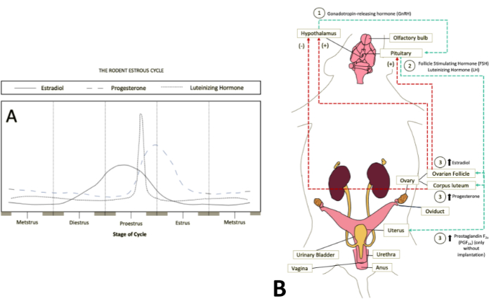
Figure 1: Hormone rhythmicity in estrous cycle stages. (A) The varying sex steroid hormone levels during the prominent estrous cycle stages are outlined and summarized. The stage progression begins and ends with metestrus to demonstrate the building hormone levels and the circular progression of the process. Adapted from an external source¹¹. (B) Flow of sex steroid hormones from the central nervous system to the reproductive system via the bloodstream. It is seen that the hormone levels are increased through signals from the hypothalamus and pituitary gland via gonadotropin-releasing hormone (GrH or LHRH) and the combination of follicle-stimulating hormone and luteinizing hormone, respectively. This includes both positive and negative feedback loops depending on the concentration of estradiol and progesterone. Information¹⁷ and images traced from external sources^65,66,67. Abbreviation: LHRH = luteinizing hormone-releasing hormone. Please click here to view a larger version of this figure.

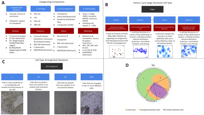
Figure 2: Estrous cycle categorizing determinants measured. (A) Listed here are the components utilized when staging the cell samples collected and the dominant components for each stage. It is important to remember that these are general parameters and differences are expected. (B) Here are the dominant cell types present in each stage. While these are general divisions, each cell type can be found within all stages. (C) Presented here are the cell arrangement types found within this study. (D) The image here reflects the typical cell quantities present in each of the 4 estrous cycle stages, with the quadrant volume representing the approximate cell quantities. Sourced from an external source¹³ and previously adapted⁶⁸. Please click here to view a larger version of this figure.

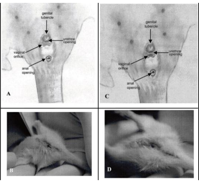
Figure 3: Vaginal opening in Sprague Dawley rats. (A) Anatomical orientation of the undeveloped external genitalia and vaginal opening that lead to the vaginal canal in relation to the urethral opening. (B) Visual representation of the undeveloped area, marked by an arrow. (C) Anatomical orientation of the developed external genitalia and vaginal orifice in relation to the urethral opening, typically occurring around 34 days of age. (D) Correspondingvisual representation of the developed area outlined in image A. All figures sourced from an external source²⁹. Please click here to view a larger version of this figure.

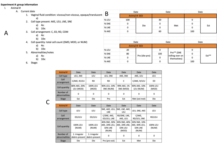
Figure 4: Categorizing determinants data recording template. (A) One option for data recording; includes descriptions of categorizing determinants. This is to be used daily, one for each rat monitored. (B) This template is an option for data entry, with a simplified recording of the categorizing determinants and rat identification. This allows for notes to be input into the datasheet in the second PRO categorization.The color on the top row reflects the color assigned to the experimental group represented, which helps distinguish one group from another. (C) Another template option; includes all categorizing determinants and can be modified based on personal preference or objectives of the study. Abbreviations: AKE = anucleated keratinized epithelial; LEU = leukocytes; LNE = large nucleated epithelial; SNE = small nucleated epithelial; C = clumped; ED = evenly dispersed; RD = randomly dispersed; COM = combined; SMD = smidge; MOD = moderate; NUM = numerous; EXE = exercise; SED = sedentary; Est = estrus; Die = diestrus; met-die = metestrus-diestrus transition; Pro = proestrus; pro-Est = proestrus-estrus transition; ** = quality example that could be helpful in a publication. Please click here to view a larger version of this figure.

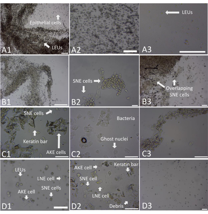
Figure 5: Stage-categorizing determinant variations. (A) This series of images depicts various examples of the diestrus stage. The first image (A1) depicts a deposit of mucus represented by strands of concentrated LEUs, with epithelial cells present in random disbursements. This is an example of the importance of utilizing both the 4x and 10x magnification. This 4x magnification appears similar to a proestrus strand but upon closer inspection at 10x, displays a dominance of LEUs. The second image (A2) depicts what was often seen in diestrus stages-a dominance of LEUs seen alongside a clumped arrangement of epithelial cells: SNE, LNE, and AKE cells. The last image in this series (A3) reflects a random disbursement of LEUs, often seen within the diestrus phase in the midst of vaginal and saline fluid droplets. (B) This series of images depicts various examples of the proestrus stage. The first image (B1) depicts a clumping arrangement of SNE cells into strands. The second image (B2) reflects a slide with a lower total cell count and a clumping of SNE cells. The third image (B3) depicts the common clumping and more random disbursement of SNE cells and low numbers of LEUs and AKE cells. (C) This series of images depicts various examples of the estrus stage. The first image (C1) depicts a common clumping arrangement of AKE cells, with keratin bar formations, in the presence of SNE cells. The second image (C2) presents the clumping of AKE cells with ghost nuclei and bacteria. The last image (C3) presents a strand-like arrangement of AKE cells. (D) This series of images depicts various examples of the metestrus stage. The first image (D1) depicts the random disbursement and clumping of LEUs, SNE cells, AKE cells, and LNE cells in the presence of debris. The second image (D2) reflects all cell types present in a clumping arrangement, alongside keratin bars. The last image (D3) shows a more comprehensive arrangement of the LEUs, SNE, AKE, and LNE cells present. These figures, taken at either 4x (A1, A2, B2, B3, D1, and D3) or 10x (A3, C1, C2, C3, and D2) objectification, have been zoomed in to allow for increased visualization of the categorization components. Scale bars = 100 μm. For size reference; AKE cells have a diameter of approximately 40-52 μm, LEUs of approximately 10 μm, LNE cells of 36-40 μm, and SNE cells of approximately 25-32 μm¹⁶. Abbreviations: SNE = small nucleated epithelial; LNE = large nucleated epithelial; AKE = anucleated keratinized epithelial; LEUs = leukocytes. Please click here to view a larger version of this figure.

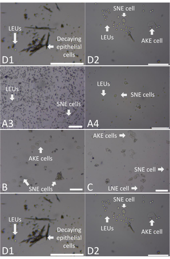
Figure 6: Transition stage samples. (A) This series of images depicts examples of the transition between the DIE and PRO stages. The first image (A1) presents large clumps and random disbursement of LEUs, SNE, LNE, and AKE cells. The second image (A2) includes a large mass of clumped LEUs and SNE with interspersed strands of LEUs. The third image (A3) includes clumps and even disbursements of LEUs and a small quantity of SNEs. The fourth and last image (A4) depicts both clumped and random disbursed SNE cells and LEUs. (B) This image depicts an example of the transition between PRO and EST stages with the clumping of SNE and AKE cells. (C) This image depicts the clumping and random disbursement of AKE, SNE, and LNE cells seen in the midst of debris to represent the transition from EST to MET. (D) The first image (D1) depicts an example of the transition between MET and DIE stages, with decaying epithelial cells accompanying an increase in LEUs. The second image (D2) depicts AKE cells in the presence of clumped LEUs and SNE cells previously described. These figures, taken at either the 4x (A1, A2, A3, B, and C) or 10x (A4, D1, and D2) magnification, have been zoomed in to allow for increased visualization of the categorization components. Scale bars = 100 m. For size reference, AKE cells have a diameter of approximately 40-52 μm, LEUs of approximately 10 μm, LNE cells of 36-40 μm, and SNE cells of approximately 25-32 μm¹⁶. Abbreviations: AKE = anucleated keratinized epithelial; LEUs = leukocytes; LNE = large nucleated epithelial; SNE = small nucleated epithelial; C = clumped; EST = estrus; DIE = diestrus; PRO = proestrus; MET = metestrus. Please click here to view a larger version of this figure.

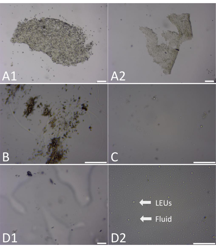
Figure 7: Unfavorable cell sample collections. (A) In these two images, squamous cells were suctioned from the vaginal canal wall, in addition to randomly dispersed LEUs. (B) This image includes a low amount of debris, where cells were either not seen or not collected. (C) In this example, a total low cell count was seen. (D) In these two images (D1 and D2), the sodium chloride (NaCl) extraction solution and vaginal fluid were seen and spread throughout the microscope slides. These figures, taken at either the 4x (A1, A2, and D1) or 10x (B, C, and D2) magnification, have been zoomed in to allow for increased visualization of the categorization components. Scale bars = 100 μm. For size reference, AKE cells have a diameter of approximately 40-52 μm, LEUs of approximately 10 μm, LNE cells of 36-40 μm, and SNE cells of approximately 25-32 μm¹⁶. Abbreviations: AKE = anucleated keratinized epithelial; LEUs = leukocytes; LNE = large nucleated epithelial; SNE = small nucleated epithelial. Please click here to view a larger version of this figure.

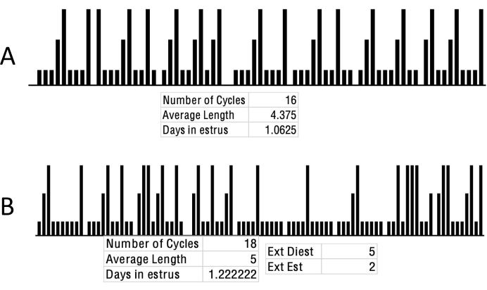
Figure 8: Regular and irregular cycling pattern sample. (A) This image reflects a total of 16 complete cycles that progress through a repetitive and consistent pattern, reflecting the regular oscillation of sex steroid hormones. Within this, diestrus is represented by the lowest, proestrus by the middle, and estrus is represented by the bar at the tallest height. These data are analyzed by tracking the days between estrus stages, with each estrus-to-estrus representing one full cycle. These data reflect data of the female rats housed at UCLA. (B) This image represents a theoretical combination of various acyclical patterns of 22 rats. Extended estrus can be seen with multiple repetitive days of bars at full height, extended diestrus seen with multiple repetitive days of the lowest bar height, and the absence of the cyclical pattern of progression from diestrus through metestrus. Abbreviations: Est = estrus; Diest/Die = diestrus. Please click here to view a larger version of this figure.

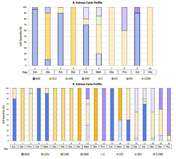
Figure 9: Individual Categorizing Determinants. (A) This stacked bar graph reflects each component of the tools utilized to categorize individual samples collected into the estrous sample stages. Here, a subject that was monitored for 10 days shows a variety of cell types, quantities, and arrangements. This is expected for adolescent animals, as hormonal levels do not typically become consistent or regularize until adulthood. (B) Here, an estrous profile is presented for an animal that was monitored for 20 days. Similar irregularities can be seen here, where the subject remained in diestrus for 4 days vs. the typical 1-2. These data represent the 6 female rats housed at Pepperdine University. Abbreviations: AKE = anucleated keratinized epithelial; LEU = leukocytes; LNE = large nucleated epithelial; SNE = small nucleated epithelial; C = clumped; ED = evenly dispersed; RD = randomly dispersed; COM = combined; SMD = smidge; MOD = moderate; NUM = numerous; EXE = exercise ; SED = sedentary; Est = estrus; Die = diestrus; Pro = proestrus; Met = metestrus.

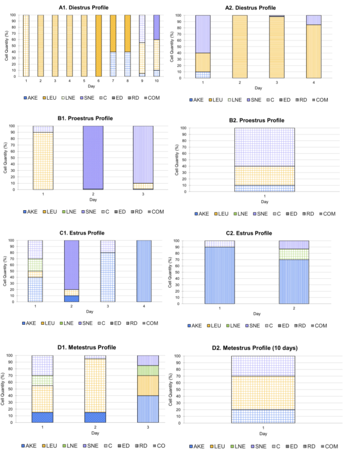
Figure 10: Stage profiles. (A) This section depicts the categorizing determinant data for individual rats during every day categorized as diestrus. The first image (A1) represents data collected over 10 days and the second (A2) for 20 days. (B) This section depicts data for individual rats during every day categorized as proestrus. The first image (B1) represents data collected over 10 days and the second (B2) for 20 days. (C) This depicts data for individual rats during every day identified as estrus stage. The first image (C1) represents data collected over 10 days and the second (C2) for 20 days. (D) This section of the series depicts the categorizing component data for individual rats during every day identified as metestrus stage. The first image (D1) represents data collected over a period of 10 days and the second (D2) for 20 days. The data in these figures reflect that of 6 female rats housed at Pepperdine University. Abbreviations: AKE = anucleated keratinized epithelial; LEU = leukocytes; LNE = large nucleated epithelial; SNE = small nucleated epithelial; C = clumped; ED = evenly dispersed; RD = randomly dispersed; COM = combined; SMD = smidge; MOD = moderate; NUM = numerous; EXE = exercise ; SED = sedentary; Est = estrus; Die = diestrus; Pro = proestrus; Met = metestrus. Please click here to view a larger version of this figure.

EST: 10 days	Duration (days)	AKE(%)	LEU (%)	LNE (%)	SNE (%)	Total Cell Count (%)
	3	88	2.78	1.89	7.33	MOD: 44.44 NUM: 44.44 SMD: 11.11
Ranges	2–4	70–100	0–10	0–17	0–20	Smidge–numerous
	Arrangement	C: 50 ED: 0 RD: 50	C: 0 ED: 0 RD: 100	C: 0 ED: 0 RD: 100	C: 50 ED: 0 RD: 50
EST: 20 days	Duration (days)	AKE(%)	LEU (%)	LNE (%)	SNE (%)	Total Cell Count (%)
	4	71.92	5.5	2.92	19.67	MOD: 50 NUM: 50 SMD: 0
Ranges	4–4	10–100	0–20	0–20	0–80	Smidge–numerous
	Arrangement	C: 60 ED: 6.67 RD: 33.33	C: 0 ED: 12.5 RD: 87.5	C: 33.33 ED: 0 RD: 66.67	C: 44.44 ED: 0 RD: 55.56

Table 1: Average stage determinant sample. These tables depict the averages for the categorizing determinants and overview for all EST stages collected. The upper table reflects the averages for all animals monitored for 10 days and the lower table for 20 days. This includes the duration of the estrous cycle, the cell types and percentages, and cell arrangements and the percentage of each arrangement seen for each cell type. These data reflect data of 6 female rats housed at Pepperdine University. Abbreviations: AKE = anucleated keratinized epithelial; LEU = leukocytes; LNE = large nucleated epithelial; SNE = small nucleated epithelial; C = clumped; ED = evenly dispersed; RD = randomly dispersed; EST = estrus.

Discussion

Key steps and important considerations
Certain critical steps in the provided protocol require emphasis, especially within the collection of vaginal cells. During the vaginal fluid extraction, ensuring the proper angle and depth of syringe insertion is key to producing satisfactory results and ultimately preventing irritation, injury, or cervical stimulation to the animal. The stimulation of the cervix can be one source of pseudopregnancy induction, indicated by 12-14 days of a leukocyte-only vaginal smear¹¹. During the microscope evaluation phase, it is crucial to focus on the visual plane displaying the vaginal cells collected. This is completed by identifying one or two cells and adjusting the visualization until focus is achieved.

Following this, capturing representative images of the vaginal cells for staging occurs by scanning the entirety of the microscope slide. This ensures that the images captured reflect an accurate portrayal of what is collected and present in the animals' vaginal canal. Before categorization, familiarity with the categorizing determinants is necessary, such as distinguishing the cell types and the various transformations each cell type can possess. It is recommended that each participant is properly trained and practices stage identification through preprepared practice slides.

To decrease the amount of bias and subjectivity involved in the process, it is recommended to include two participants in the categorizing phase, both remaining blind to the treatment group assignments while knowing previously recorded stage identifications for each animal. Assigning two participants to categorize samples allows for conference and a decrease in subjectivity in the identifications. However, if the participants are to categorize samples separately, it is recommended that there is an initial collaboration period to increase inter-rater reliability as expertise is developed. A secondary examination system can be employed to prevent inconsistent findings, such as exchanging data sets after categorization and utilizing the photos to confirm the initial assessments.

Limitations and modifications
Limitations of the current technique include the duration of viability. Due to the injury or irritation that could accompany repetitive insertion of a syringe, prolonged and recurrent monitoring does not align with proper care and use of animals. Therefore, when performing a longitudinal study, it may be necessary to modify the procedure by decreasing the frequency of the lavage. For instance, rather than monitoring each animal once per day, the rats could be divided into groups monitored on different days throughout the week. A second limitation involves the absence of sample staining in the process outlined, with no separation of cellular components by color, creating a greater reliance on the categorization determinants listed in the protocol above.

In addition, within such categorization determinants, there are elements of subjectivity that could limit precise replication. Specifically, the cell quantity percentages within samples collected are based on personal estimations. Modifications in this regard could include developing a mathematical algorithm to quantify the individual cell types present. Alternative modifications could include the number of samples deposited onto one microscope slide, which could be increased depending on the size of the slide and cover. Further limitations could include the lack of vaginal fluid data in this study—a modification of future studies could include recording the conditions of the vaginal fluid collected as a contribution to stage categorization. Additional modifications of the protocol could include utilizing another isotonic fluid for cell extraction, which would produce the same results, such as phosphate-buffered saline¹³. Lastly, when applying this procedure to rats of different ages or strains, modifications such as animal handling techniques may be required due to body size or activity level. This can include the grasping method⁶⁹ and the Forelimb Crisscross⁶⁴ methods for adults and the One- and Two-handed Restraint⁶⁴ method utilized for younger rats.

Alternative methods
Compared to alternative methods of estrous cycle monitoring, the vaginal lavage is unique in its accuracy, amount of information produced, minimal invasiveness, and low associated costs. The histological examination of the uterus and ovaries can be utilized to identify cycle stages but is more intrusive and does not allow continual monitoring. While measuring the sex steroid hormone levels assists with monitoring the estrous cycle, it requires blood collection and does not allow for the characterization of the unique cellular or vaginal fluid profile of each subject. As the development of external genitalia is indirectly correlated with sex steroid hormone levels, the examination of the vaginal opening can provide information on sexual maturation. Additionally, the coloration of the tissue, level of moisture, size, and swelling of the vaginal opening has been correlated with the estrous cycle stages⁷⁰. However, the precise physiology leading to the opening of the vaginal canal in rats has yet to be fully reported. Recent publications have found that this is only an indirect marker of reproductive development and does not always align with pubescence^31,34. The biochemical analysis of urine samples is cost-effective and easily conducted, but does not allow for the specificity and reliability of other methods⁷¹. Therefore, it is not as reliable or valid as examining the cells present in the vaginal canal.

Additionally, the measurement of electrical impedance has been utilized to monitor the estrous cycle and is less physically irritating than the liquid lavage. However, this method does not provide as much information on the categorizing components. This device is specifically designed to optimize the timing of intentional mating, measuring when sex steroid hormone levels are highest^72,73,74. Additionally, it has been reported that this method is effective for distinguishing between EST and nonEST but is limited in its ability to monitor the estrous cycle outside of that⁷⁵. Overall, this method has been reported to be unreliable, not always cost-effective, and is not often utilized in the literature leading to a lack of comparable data⁷⁴. While the vaginal swab is most similar to the lavage in the information it provides, it includes an increased risk of irritation or injury as it requires contacting the lining of the vaginal canal directly to retrieve cells. Lastly, while staining the microscope slides may provide a sharper contrast between cell types and allow for sample preservation, it is a more time-consuming and costly endeavor than the wet mount⁵³. Overall, each monitoring technique has its limitations and advantages, and it could be beneficial to utilize a combination of these methods to receive a comprehensive examination of the rodent estrous cycle.

Applications
It remains important to view the current study in the context of the greater scientific community and the general public. This methodology can be utilized in any project that involves examining female animals—not solely within studies focusing on intentional breeding, to exclude animals that present with abnormalities, and/or the function of the hypothalamic-pituitary-ovarian axis, but also for principal insights within treatment groups. More specifically, this procedure is impactful within i) pharmacological studies, as various medications and chemicals disrupt or alter the reproductive tract and estrous cycle^11,27,76; ii) neurological studies, such as those focused on traumatic brain injuries, cognition, or degenerative disorders, due to interactions between sex steroid hormones and the nervous system⁷⁷; iii) circulatory system research due to sex steroid hormone receptors located on myocytes and the subsequent interactions⁷⁷; iv) research related to bone growth³⁸; to the endocrine system^11,78; and v) other nonreproductive studies³.

Materials

Name	Company	Catalog Number	Comments
AmScope 40X-1000X LED Student Microscope + 5MP USB Camera	AmScope	Part Number: M150C-E5 EAN: 0608729747796 Model Number: M150C-E5	https://www.amazon.com/AmScope-40X-1000X-Student-Microscope-Camera/dp/B00O9GNOTA/ref=sr_1_15?crid=2W9CHTG8YSOTV& keywords=usb+camera+for+microscope& qid=1572477663&s=industrial &sprefix=USB+camera+for+micr%2Cindustrial%2C177&sr=1-15
BD PrecisionGlide Needle Pack, 20G x 1, Short Bevel	Fischer Scientific	14-815-526	https://www.fishersci.com/shop/products/bd-precisionglide-single-use-needles-short-bevel-regular-wall-4/14815526#?keyword=BD%20PrecisionGlide%20Needle%20Pack,%2020G%20x%201
Bed O Cob 1/8	NEWCO	93009	https://andersonslabbedding.com/cob-products/bed-ocobs-8b/
Corning™ Plain Microscope Slides Plain water-white glass	Fischer Scientific	12-553-7A	https://www.fishersci.com/shop/products/corning-plain-microscope-slides-microscope-slides-75-x-25mm/125537a
Corning™ Rectangular Cover Glasses	Fischer Scientific	12-553-464	https://www.fishersci.com/shop/products/corning-square-rectangular-cover-glasses-rectangle-no-1-thickness-0-13-0-17mm-size-24-x-50mm/12553464#?keyword=true
Kimberly-Clark Professional™ Kimtech Science™ Kimwipes™ Delicate Task Wipers, 1-Ply	Fischer Scientific	06-666	https://www.fishersci.com/shop/products/kimberly-clark-kimtech-science-kimwipes-delicate-task-wipers-7/p-211240?crossRef=kimwipes
Labdiet Rodent Lab Chow 50lb, 15001	NEWCO Specialty and LabDiet	5012	https://www.labdiet.com/products/standarddiets/rodents/index.html
Linear LED Bulb, UL Type A, T8, Medium Bi-Pin (G13), 4,000 K Color Temperature, Lumens 2550 lm	Grainger	36UX10	https://www.grainger.com/product/36UX10?gclid=CjwKCAjw_ LL2BRAkEiwAv2Y3SW1WdNdkf7 zdIxoT9R6n2DGnrToJHjv-pwCTca4ahQyExrrtWvbgwRoCi4 cQAvD_BwE&s_kwcid=AL!2966!3!335676016696 !p!!g!!led18et8%2F4%2F840&ef_id= CjwKCAjw_LL2BRAkEiwAv2Y3SW 1WdNdkf7zdIxoT9R6n2DGnrToJ Hjv-pwCTca4ahQyExrrtWvbgwRo Ci4cQAvD_BwE:G:s&s_kwcid=AL!2966!3!335676016696!p!!g!!led18et8%2F4%2F840&cm_mmc= PPC:+Google+PPC
Sodium Chloride Injection Bags, 0.9%	Live Action Safety	ABB079830939	https://www.liveactionsafety.com/injection-iv-solution-9-sodium-chloride-1000ml-bags/
Syringe Sterile 1ml  with Luer Slip Tip - 100 Syringes by BH Supplies	BH Supplies	ASIN: B07BQDRDC2 UPC: 638632928821	https://www.amazon.com/1ml-Syringe-Sterile-Luer-Slip/dp/B07BQDRDC2/ref=sr_1_1_sspa?crid=13S8EGEUK90G7& keywords=1ml+sterile+syringe&qid= 1572478649&s=industrial &sprefix=1+ml+steri%2Cindustrial%2C187&sr=1-1-spons&psc=1&spLa= ZW5jcnlwdGVkUXVhbGlmaWVy PUEyRlo4NFdZWkJLWkxGJm VuY3J5cHRlZElkPUEwMDEzODQ yMjNWNzdWM0hTNzVBRCZlbmNy eXB0ZWRBZElkPUEwNDI3NzAzM 0E5SzVKMkxaQVc2JndpZGdldE5h bWU9c3BfYXRmJmFjdGlvbj1jbGlja 1JlZGlyZWN0JmRvTm90TG9nQ2 xpY2s9dHJ1ZQ==
Wire lids and floors Mouse Maternity Wire Bar LidUsed with Rat Cage (10" X 19" x 8"H )Overall dimen	Allentown	LV40326013	https://www.labx.com/item/wire-lids-and-floors-mouse-maternity-wire-bar-lidused/LV40326013#description
Ultra Lightweight Tissue and Plastic 17' x 24' Disposable Underpad	Medline	EAN: 0480196288558  Global Trade Identification Number: 40080196288558	https://www.amazon.com/Medline-Industries-MSC281224C-Lightweight-Disposable/dp/B00A2G67YU/ref=sr_1_4?keywords=medline+industries+surgical+pads&qid=1572475853& sr=8-4